CONSTRAINED OPTIMIZATION How much land can a person enclose? Can run - PowerPoint PPT Presentation
ECO 300 FALL 2005 September 20 CONSTRAINED OPTIMIZATION How much land can a person enclose? Can run length L in a day (not necessarily integer) Chooses rectangle of width x , height y subject to constraint: 2 x + 2 y = L Wants to maximize
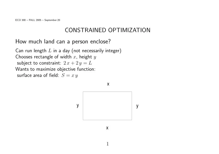
ECO 300 – FALL 2005 – September 20 CONSTRAINED OPTIMIZATION How much land can a person enclose? Can run length L in a day (not necessarily integer) Chooses rectangle of width x , height y subject to constraint: 2 x + 2 y = L Wants to maximize objective function: surface area of field: S = x y 1
MAT 103 approach: Substitute for y from constraint to express S in terms of just one choice variable x : � L = L � 2 x − x 2 S = x 2 − x Graph of function shown for L = 40 : 2
Optimal x found using first-order condition dS dx = L 2 − 2 x = 0 Also check second-order condition: d 2 S dx 2 = − 2 < 0 Solution: x = L/ 4 ; best rectangle is a square. Resulting area: S = L 2 / 16 If shape is not restricted to rectangle, true optimum is circle � L � 2 Radius = L = L 2 L 2 2 π, Area = π 4 π ≈ 2 π 12 . 57 3
Economically useful information: Average product AP = S/L = L/ 16 Marginal product MP = dS/dL = 2 L/ 16 = L/ 8 Notes: (1) AP and MP are upward-sloping: system has “increasing returns”, (2) Slope of MP = 2 * Slope of AP (because AP curve is a straight line) 4
ECO 100 approach: Draw picture showing constraint, and contours or level curves of objective function x y = constant curves are rectangular hyperbolas Figure shows numerical solution for L = 40 5
Look for highest attainable level curve Along any curve y = constant /x , Slope (Marginal rate of substitution) = − constant /x 2 = − x y/x 2 = − y/x Slope of constraint = − 1 Condition of tangency − y/x = − 1 Therefore y = x , and x + y = 20 So optimal x = y = 10 , S = 100 Observe similarity to consumer theory (budget line and indifference curves) Will use your knowledge of this, and relate it to the other two approaches 6
Lagrange’s Method: Suppose instead of fixed number of miles L the person can buy miles at price p measured in units of land area itself Net amount of land (profit) Π = x y − p (2 x + 2 y ) To choose x , y to maximize Π : Take derivatives Π with respect to x , y one at a time, holding the other constant Set both of these “partial” derivatives equal to 0 ∂ Π ∂ Π ∂x = y − 2 p = 0 , ∂y = x − 2 p = 0 So x = y = 2 p , total “demand for length” 2 x + 2 y = 8 p 7
Relate this to previous work: Actually L is fixed, so find p such that the person will want to use exactly L i.e. “demand” 8 p equals “supply” L So 8 p = L , or p = L/ 8 Then x = y = L/ 4 , and S = L 2 / 16 p is called Lagrange multiplier and profit expression is called the Lagrangian Note p = dS/dL , marginal product This is “implied value” of the constraint – possible benefit if constraint can be relaxed a little Equals maximum willingness to pay to get it relaxed 8
Hence usefulness of this approach Other applications later (1) Firm minimizes cost of producing a specified level of output Lagrange multiplier = marginal cost of production (2) Consumer maximizes utility subject to budget constraint (limited money income) Lagrange multiplier = marginal utility of money Thus Lagrange’s method useful throughout economics In P–R textbook, see Appendixes to Chapters 4, 7 9
(Honest disclosure – the “profit-max” interpretation above involves some cheating second-order condition for profit-max not satisfied because system has increasing returns If you could see this, go to ECO 310 Otherwise do not worry about this issue Correct math second-order condition different and difficult, involves “mercenary matrices” called “bordered Hessians” So math solution correct, but not profit-max analogy We will actually use profit-max only for diminishing returns systems, so interpretation will be correct) 10
Recommend
More recommend
Explore More Topics
Stay informed with curated content and fresh updates.
