Connection Preserving Deformation Approach to the Q-Difference - PowerPoint PPT Presentation

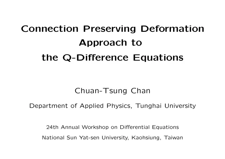
Connection Preserving Deformation Approach to the Q-Difference Equations Chuan-Tsung Chan Department of Applied Physics, Tunghai University 24th Annual Workshop on Differential Equations National Sun Yat-sen University, Kaohsiung, Taiwan

Mindset of this Study • Physics: Theory of theories – Notion of universality classes from the physics of phase transitions and critical phenomena. – Landscape/multiverse picture as inferred from the study of quan- tum gravity. – M theory (or even higher structure) as a unified arena of string theories. • Mathematics: Structure of structures – Classifications of algebraic and geometrical structures. – Classifications of differential equations. – Langlands Program as a GUT in mathematics.

Outline of this Talk 1. Introduction and Motivation 2. Discrete Painlev´ e Equations 3. Linear Q-difference Equations and Connection Preserving Deformation (CPD) 4. Derivation of Q-discrete PVI Equation based on Connection Preserving Deformation 5. Generalization to the Lax Pair of Jordan Type 6. Summary

Part I Introduction and Motivation

Architects of the Modern Theories of ODEs Paul Painlev´ e Lazarus Fuchs (1863-1933) (1833-1902)

Continuous Painlev´ e Equations d 2 y dt 2 = 6 y 2 + t (1) d 2 y dt 2 = 2 y 3 + ty + α (2) tyd 2 y � 2 � dy − ydy dt + δt + βy + αy 3 + γty 4 dt 2 = t (3) dt yd 2 y � 2 dt 2 = 1 + β + 2( t 2 − α ) y 2 + 4 ty 3 + 3 � dy 2 y 4 (4) 2 dt � 1 d 2 y � 2 1 �� dy − 1 dy dt 2 = 2 y + y − 1 dt t dt + ( y − 1) 2 t + δy ( y + 1) αy + β + γy � � (5) t 2 y y − 1 d 2 y � 2 dt 2 = 1 � 1 1 1 �� dy � 1 1 1 � dy y + y − 1 + t + t − 1 + − 2 y − t dt y − t dt + y ( y − 1)( y − t ) ( y − 1) 2 + δt ( t − 1) t − 1 α + β t � � y 2 + γ (6) t 2 ( t − 1) 2 ( y − t ) 2

Specialities about the Painlev´ e Equations 1. The list were corrected and completed by B. Gambier and R. Fuchs. 2. They are ”exceptional cases (6 out of 50)” in the classifications of the 2nd order differential equations which admit ”Painlev´ e property”, and the general solutions can not be expressed in terms of ”standard functions”. The only movable singularities of the solutions to these eqs. are poles! 3. They can be derived as characterizations of isomonodromy deforma- tions of systems of linear ordinary differential equations. The most general form of PVI (6th Painlev´ e eq.) was discovered by Richard Fuchs in 1905 through this approach. e.g., P-Q systems of the string equations. 4. They appear in many physical systems of fundamental importance. e.g., correlators in the statistical model (e.g., Ising model), susceptibility of free-energy of 2-dim gravity/matrix model.

Part II Discrete Painlev´ e Equations

Some Pioneers of the Discrete Painlev´ e Equations A. Ramani B. Grammaticos J. Hietarinta

Discrete Painlev´ e Equations x n +1 + x n − 1 + x n = an + b + c (7) x n x n +1 + x n − 1 = x n ( an + b ) + c (8) 1 − x 2 n x n − 1 x n +1 = γx 2 n + ζ 0 λ n x n + µ 0 λ 2 n (9) x 2 n + βx n + γ n + [ ǫ 0 − 1 x n +1 x n − 1 + x n ( x n +1 + x n − 1 ) = − ( an + b ) x 3 4 ( an + b ) 2 ] x 2 n + µ n + ( an + b ) x n + [ γ 0 + 1 x 2 4 ( an + b ) 2 ] (10) (2 x n − 1) x n +1 x n − 1 − x n ( x n +1 + x n − 1 ) = 4 ( σ + α 0 λ 2 n − 2 ρ 0 λ n ) } x 2 1 n + { θ + 1 2 ( σ − α 0 λ 2 n ) x 3 n − 2 µx n + µ (11) n + ( ρ 0 λ n − α 0 λ 2 n ) x n + 1 4 ( σ + α 0 λ 2 n − 2 ρ 0 λ n ) α 0 λ 2 n x 2

Basics of the Singularity Confinement Test Starting from the QRT (Quispel, Roberts, and Thompson) class of the second order difference equations, f 3 ( x n ) · Π − f 2 ( x n ) · Σ + f 1 ( x n ) = 0 , with Π := x n − 1 · x n +1 , Σ := x n − 1 + x n +1 , and f i are quartic polynomials . A. Ramani, B. Grammaticos, and J. Hietarinta identified a criterion, in parallel to the sprit of Painlev´ e property, that if there exists an instance where the solution of a difference equation diverges, it will only last for a finite iterations and beyond this finite interval, the solution will become regular and restores the memory of previous data. Hence the name singularity confinement .

IV Hermite-Weber V Kummer III Bessel I None II Airy VI Gauss Specialities of the Discrete Painlev´ e Equations 1. Painlev´ e equations (continuous and discrete) follow the same conflu- ence/degeneration pattern as that of the hypergeometric equations: 2. Conceptual issue : How much can we trust calculus as a useful language for a description of the microscopic world? e.g., quantum theories are inherently discrete? 3. Pragmatic issue : How do we implement the integrability properties in the numerical computations of the integrable differential equations? 4. Are there any guiding principle for a characterization/classification of ordinary difference equations?

Connection Preserving Deformation Discrete Painlevé Equations Matrix Models at finite N and k-cuts Interconnection and Motivation

Part III Linear Q-Difference Equations and Connection Preserving Deformation

Architects of the Isomonodromy Theories Michio Jimbo Tetsuji Miwa

Linear Q-Difference Equations a l´ a Birkhoff • Definition of q-differentiation symbol (acting on a matrix function): D q Y ( x ) := Y ( qx ) − Y ( x ) , q := 1 − ǫ. qx − x • Consider a 2 × 2 matrix system with polynomial coefficients A ( x ) = A 0 + A 1 + ... + A N x N . Y ( qx, q ) = A ( x ) Y ( x, q ) , Assumptions: A 0 , A N are both semi-simple and invertible, and their eigenvalues are θ j and κ j , j = 1 , 2 . • Diagonalization of the coefficient matrices: A 0 = C 0 q D 0 C − 1 A ∞ = C ∞ q D ∞ C − 1 0 , ∞ where D 0 := diag (ln θ j / ln q ) , D ∞ := ≡ diag (ln κ j / ln q )

Asymptoes of the solutions near boundaries • The unique solution to the q-difference equation is fixed by the asymptotic behaviours : u := ln x N Y 0 ( x ) x D 0 , 2 u ( u − 1) ˆ Y ∞ ( x ) x D ∞ , Y 0 ( x ) = ˆ Y ∞ ( x ) = q ln q • Subleading contributions: ˆ Y 0 ( x ) is a holomophic and invertible matrix at x = 0, with ˆ Y 0 (0) = C 0 , and ˆ Y ∞ ( x ) is a holomophic and invertible matrix at x = ∞ , with ˆ Y ∞ ( ∞ ) = C ∞ . • The degeneration point of the coefficient matrix A ( x ), det A ( α j ) = 0 , j = 1 , ..., 2 N. may induce poles of the subleading parts of the asymptotic solutions: Y ∞ ( x ) − 1 : qα j , q 2 α j , q 3 α j , ...... Y 0 ( x ) : , α j q − 1 α j , q − 2 α j , ...... ˆ ˆ

Connection Matrix and the Lax Pair • Definition of the connection matrix: P ( x ) := Y ∞ ( x )[ Y 0 ( x )] − 1 . • Introducing a deformation parameter, t , such that Y ( qx, t ) = A ( x, t ) Y ( x, t ) , and P ( x ) → P ( x, t ) • Definition of the dual operator: B ( x, t ) := Y ( x, qt )[ Y ( x, t )] − 1 , A ( x, t ) and B ( x, t ) are the Lax pair of the linear q-difference system. • Proposition: Connection preserving deformation fixes dual operator to be a rational function! In the case of N = 2, we get x ( xI + B 0 ( x )) P ( x, qt ) = P ( x, t ) ↔ B ( x, t ) = ( x − qta 1 )( x − qta 2 )

From Compatiblility Condition to the Discrete Painlev´ e VI Equation From this commuting diagram, we have the following constraint on the Lax pair, A ( x, qt ) · B ( x, t ) = B ( qx, t ) · A ( x, t ) .

Part IV Derivation of Q-discrete PVI Equation based on Connection Preserving Deformation

General Parametrization of the Linear System (I) • Recall the definition of the coefficient matrix ( N = 2): A ( x, t ) = A 0 ( t ) + A 1 ( t ) x + A 2 x 2 (12) � � κ 1 0 A 2 = , A 0 ( t ) has eigenvalues tθ 1 , tθ 2 0 κ 2 det A ( x, t ) = κ 1 κ 2 ( x − ta 1 )( x − ta 2 )( x − a 3 )( x − a 4 ) , (13) 4 � with κ 1 κ 2 a j = θ 1 θ 2 . (14) j =1 • Define the Painlev´ e functions: z 1 ( t ) := A 11 ( y ( t ) , t ) z 2 ( t ) := A 22 ( y ( t ) , t ) A 12 ( y ( t ) , t ) = 0 , , , κ 1 κ 2 and z = ( y − ta 1 )( y − ta 2 ) (15) qκ 1 z 1 � � κ 1 (( x − y )( x − α ) + z 1 ) κ 2 w ( x − y ) A ( x, t ) = (16) κ 1 w − 1 ( γx + δ ) κ 2 (( x − y )( x − β ) + z 2 )

Compatibility Conditions of the Linear System ⇒ q-PVI • Constraint among y, z 1 , z 2 : det A ( y ( t ) , t ) = z 1 ( t ) · z 2 ( t ). z 1 · z 2 = ( y − ta 1 )( y − ta 2 )( y − a 3 )( y − a 4 ) ⇒ Only y ( t ) and z ( t ) are independent Painlev´ e functions! • Reducing the unknowns: α, β, γ, δ can be expressed by – eigenvalue datum of A 2 , and A 0 : κ j , θ j , j = 1 , 2 . – degeneration points of A ( x ): a 1 , a 2 , a 3 , a 4 . – Painlev´ e functions y ( t ), and z ( t ). through the det A ( x, t ) and tr A ( x, t ) relations. • Compatibility condition among the Lax pair A ( x, t ) , B ( x, t ) leads to – Solution of the B 0 ( t ) in the dual evolution operator B ( x, t ). – Coupled first order difference equations in three unknown func- tions, y ( t ) , z ( t ) , w ( t ). ⇒ d-PVI equation in the first order form!

Discrete Q-PVI Equations in the first order form y ¯ y = (¯ z − tb 1 )(¯ z − tb 2 ) z − b 4 ) , (17) (¯ z − b 3 )(¯ a 3 a 4 z ¯ z = ( y − ta 1 )( y − ta 2 ) (18) ( y − a 3 )( y − a 4 ) , b 3 b 4 w w = b 4 ¯ z − b 3 ¯ (19) b 3 ¯ z − b 4 1 b 4 = 1 b 1 = a 1 a 2 b 2 = a 1 a 2 b 1 b 2 = qa 1 a 2 b 3 = (20) , , , , θ 1 θ 2 qκ 1 κ 2 b 3 b 4 a 3 a 4

Part V Generalization to the Lax pair of Jordan Type