12.1 Surface Deformation II Hao Li http://cs621.hao-li.com 1 Last - PowerPoint PPT Presentation

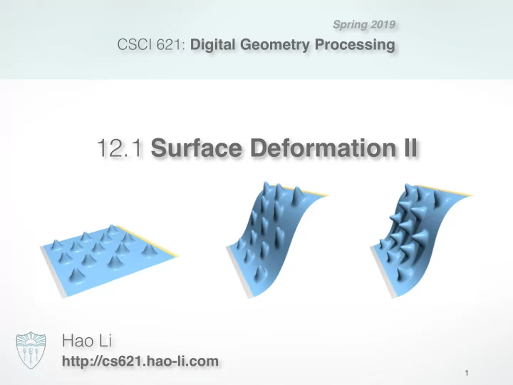
Spring 2019 CSCI 621: Digital Geometry Processing 12.1 Surface Deformation II Hao Li http://cs621.hao-li.com 1

Last Time Linear Surface Deformation Techniques • Shell-Based Deformation • Multiresolution Deformation • Differential Coordinates 2

Nonlinear Surface Deformation • Nonlinear Optimization • Shell-Based Deformation • (Differential Coordinates) 3

Nonlinear Optimization • Given a nonlinear deformation energy E ( d ) = E ( d 1 , . . . , d n ) find the displacement d ( x ) that minimizes E ( d ) , while satisfying the modeling constraints. • Typically E ( d ) stays the same, but the modeling constraints change each frame. 4

Gradient Descent • Start with initial guess d 0 • Iterate until convergence – Find descent direction h = - ∇ E ( d ) – Find step size λ – Update d = d + λ h • Properties + Easy to implement, guaranteed convergence – Slow convergence 5

Newton’s Method • Start with initial guess d 0 • Iterate until convergence – Find descent direction as H ( d ) h = - ∇ E ( d ) – Find step size λ – Update d = d + λ h • Properties + Fast convergence if close to minimum – Needs pos. def. H , needs 2 nd derivatives for H 6

Nonlinear Least Squares Given a nonlinear vector-valued error function   e 1 ( d 1 , . . . , d n ) . . e ( d 1 , . . . , d n ) =   .   e m ( d 1 , . . . , d n ) find the displacement d ( x ) that minimizes the nonlinear least squares error E ( d 1 , . . . , d n ) = 1 2 � e ( d 1 , . . . , d n ) � 2 7

1st order Taylor Approximation E ( d 1 , . . . , d n ) = 1 2 � e ( d 1 , . . . , d n ) � 2 k e ( d k +1 ) k 2 ⇡ k e ( d k ) + J e ( d k +1 � d k ) k 2 Taylor Approx k e ( d k +1 ) k 2 ⇡ k e ( d k ) + J e ∆ d k k 2 ∆ d k ∆ d k k e k 2 min = arg min Gauss-Newton ∆ d k k e k 2 h = arg min J > e J e h = − J > e e ( d k ) 8

Gauss-Newton Method • Start with initial guess d 0 • Iterate until convergence – Find descent direction as ( J ( d ) T J ( d )) h = - J ( d ) T e – Find step size λ – Update d = d + λ h • Properties + Fast convergence if close to minimum – Needs full-rank J ( d ) , needs 1 st derivatives for J ( d ) 9

Nonlinear Optimization • Has to solve a linear system each frame – Matrix changes in each iteration! – Factorize matrix each time • Numerically more complex – No guaranteed convergence – Might need several iterations – Converges to closest local minimum ➡ Spend more time on fancy solvers... 10

Nonlinear Surface Deformation • Nonlinear Optimization • Shell-Based Deformation • (Differential Coordinates) 11

Shell-Based Deformation • Discrete Shells [Grinspun et al, SCA 2003] • Rigid Cells [Botsch et al, SGP 2006] • As-Rigid-As-Possible Modeling [Sorkine & Alexa, SGP 2007] 12

Discrete Shells • Main idea – Don’t discretize continuous energy – Define discrete energy instead – Leads to simpler (still nonlinear) formulation • Discrete energy – How to measure stretching on meshes? – How to measure bending on meshes? 13

Discrete Shell Energy • Stretching : Change of edge lengths e ij | ) 2 � λ ij ( | e ij | − | ¯ e ij ∈ E x k x j f ijk • Stretching : Change of triangle areas e ij ⇤⇥ 2 ⌅ f ilj ⇤ ⇤ � ⇤ ¯ | f ijk | − λ ijk f ijk x i f ijk ∈ F x l • Bending : Change of dihedral angles ⇥ 2 ⇤ � θ ij − ¯ θ ij µ ij e ij ∈ E 14

Discrete Shell Energy 15

Realistic Facial Animation Linear model Nonlinear model 16

Discrete Energy Gradients • Gradients of edge length | e ij | ⇤ x j � x i ⇤ = ∂ | e ij | � e = ⇤ e ⇤ ∂ x i n 1 x k x j ∂ | e ij | e = ⇤ e ⇤ ∂ x j n 2 e x i x l 17

Discrete Energy Gradients • Gradients of triangle area 1 | f ijk | = 2 ⌅ n 1 ⌅ ∂ | f ijk | n 1 ⇥ ( x k � x j ) = 2 ⌅ n 1 ⌅ ∂ x i n 1 ∂ | f ijk | n 1 ⇥ ( x i � x k ) x k = x j 2 ⌅ n 1 ⌅ ∂ x j n 2 ∂ | f ijk | n 1 ⇥ ( x j � x i ) e = 2 ⌅ n 1 ⌅ ∂ x k x i x l 18

Discrete Energy Gradients • Gradients of dihedral angle � sin θ ⇤ ⌅ ( n 1 ⇤ n 2 ) T e ⇥ = atan = atan θ n T cos θ 1 n 2 · ⌅ e ⌅ ( x k � x j ) T e ⌅ n 1 ⌅ 2 + ( x l � x j ) T e · � n 1 · � n 2 ∂θ = ⌅ n 2 ⌅ 2 ⌅ e ⌅ ⌅ e ⌅ ∂ x i n 1 ( x i � x k ) T e ⌅ n 1 ⌅ 2 + ( x i � x l ) T e · � n 1 · � n 2 ∂θ x k = x j ⌅ n 2 ⌅ 2 ⌅ e ⌅ ⌅ e ⌅ ∂ x j ∂θ ⌅ e ⌅ · � n 1 n 2 = e ⌅ n 1 ⌅ 2 ∂ x k ⌅ e ⌅ · � n 2 ∂θ x i = ⌅ n 2 ⌅ 2 ∂ x l x l 19

Discrete Shell Editing • Problems with large deformation – Bad initial state causes numerical problems 20

Shell-Based Deformation • Discrete Shells [Grinspun et al, SCA 2003] • Rigid Cells [Botsch et al, SGP 2006] • As-Rigid-As-Possible Modeling [Sorkine & Alexa, SGP 2007] 21

Nonlinear Shape Deformation • Nonlinear editing too unstable? • Physically plausible vs. physically correct ➡ Trade physical correctness for – Computational efficiency – Numerical robustness 22

Elastically Connected Rigid Cells • Qualitatively emulate thin-shell behavior • Thin volumetric layer around center surface • Extrude polygonal cell C i per mesh face 23

Elastically Connected Rigid Cells • Aim for robustness – Prevent cells from degenerating ➡ Keep cells rigid 24

Elastically Connected Rigid Cells • Connect cells along their faces – Nonlinear elastic energy – Measures bending, stretching, twisting, ... 25

Notion of Prism Elements 26

Nonlinear Minimization • Find rigid motion T i per cell C i ⇧ ⇤ 2 d u ⌅ f i → j ( u ) f j → i ( u ) ⇤ ⇥⇤ � ⇥ � min ⇤ T i − T j w ij { T i } { i,j } [0 , 1] 2 • Generalized global shape matching problem – Robust geometric optimization – Nonlinear Newton-type minimization – Hierarchical multi-grid solver 27

Newton-Type Iteration 1. Linearization of rigid motions R i x + t i x + ( ω i × x ) + v i =: A i x ≈ 2. Quadratic optimization of velocities ⇤ 2 d u ⇧ ⌅ f i → j ( u ) f j → i ( u ) ⇤ ⇥⇤ � ⇥ � min ⇤ A i − A j w ij { v i , ω i } { i,j } [0 , 1] 2 3. Project A i onto rigid motion manifold ➡ Local shape matching R i P i P i + t i A i ( P i ) 28

Robustness 29

Character Posing 30

Goblin Posing • Intuitive large scale deformations • Whole session < 5 min 31

Shell-Based Deformation • Discrete Shells [Grinspun et al, SCA 2003] • Rigid Cells [Botsch et al, SGP 2006] • As-Rigid-As-Possible Modeling [Sorkine & Alexa, SGP 2007] 32

Surface Deformation • Smooth large scale deformation • Local as-rigid-as-possible behavior – Preserves small-scale details 33

Cell Deformation Energy • Vertex neighborhoods should deform rigidly ⇤ 2 → min ⌅ ⇤ ⇤ ⇤� ⇥ p � j − p � − R i ( p j − p i ) i j ⇥ N ( i ) p i p j 34

Cell Deformation Energy • If p , p ′ are known then R i is uniquely defined R i p � p i i p � p j j • Shape matching problem – Build covariance matrix S = PP ′ T – SVD: S = U Σ W T – Extract rotation R i = UW T 35

Total Deformation Energy • Sum over all vertex n ⇤ 2 ⌅ ⌅ ⇤ ⇤ ⇤� ⇥ p � j − p � min − R i ( p j − p i ) i p � i =1 j ⇥ N ( i ) • Treat p ′ and R i as separate variables • Allows for alternating optimization – Fix p ′ , find R i : Local shape matching per cell – Fix R i , find p ′ : Solve Laplacian system 36

As-Rigid-As-Possible Modeling • Start from naïve Laplacian editing as initial guess initial guess 1 iteration 2 iterations initial guess 1 iterations 4 iterations 37

As-Rigid-As-Possible Modeling 38

Shell-Based Deformation • Discrete Shells [Grinspun et al, SCA 2003] • Rigid Cells [Botsch et al, SGP 2006] • As-Rigid-As-Possible Modeling [Sorkine & Alexa, SGP 2007] 39

Nonlinear Surface Deformation • Limitations of Linear Methods • Shell-Based Deformation • (Differential Coordinates) 40

Subspace Gradient Deformation • Nonlinear Laplacian coordinates • Least squares solution on coarse cage subspace [Huang et al, SIGGRAPH 06] 41

Mesh Puppetry • Skeletons and Laplacian coordinates • Cascading optimization [Shi et al, SIGGRAPH 07] 42

Nonlinear Surface Deformation • Limitations of Linear Methods • Shell-Based Deformation • (Differential Coordinates) 43

Linear Approaches Nonlinear Energy Linearization Quadratic Energy Variational Calculus Linear PDE Discretization Linear Equations 44

Linear Approaches • Resulting linear systems – Shell-based ∆ 2 d = 0 – Gradient-based ∆ p = ⇥ · T ( g ) – Laplacian-based ∆ 2 p = ∆ T ( l ) • Properties – Highly sparse – Symmetric, positive definite ( SPD ) – Solve for new RHS each frame! 45