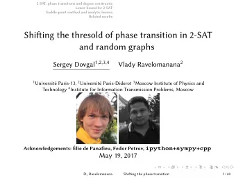
Shifing the thresold of phase transition in 2-SAT and random graphs - PowerPoint PPT Presentation
Problem and Motivation Saddle-point method and analytic lemma Distribution of random parameters Lower bound for 2-SAT Shifing the thresold of phase transition in 2-SAT and random graphs Sergey Dovgal 1 , 2 Vlady Ravelomanana 2 1 Universit
Problem and Motivation Trees with degree constraints Saddle-point method and analytic lemma Unicycles with degree constraints Distribution of random parameters Kernel of a graph Lower bound for 2-SAT General symbolic lemma Trees with degree constraints Unrooted case Excercise A variant of dissymmetry theorem: • • • 1 • • = + + ◦ 1 ◦ 1 (∆) T 0 ( z ) = T 1 ( z ) 2 U ( z ) = T 0 ( z ) − T 1 ( z ) 2 + U ( z ) ⇔ 2 2 D., Ravelomanana Shifing the phase transition 12 / 51
Problem and Motivation Trees with degree constraints Saddle-point method and analytic lemma Unicycles with degree constraints Distribution of random parameters Kernel of a graph Lower bound for 2-SAT General symbolic lemma Unicycles with degree constraints Excercise ≥ 3 Excercise: what is the EGF for unicycles? D., Ravelomanana Shifing the phase transition 13 / 51
Problem and Motivation Trees with degree constraints Saddle-point method and analytic lemma Unicycles with degree constraints Distribution of random parameters Kernel of a graph Lower bound for 2-SAT General symbolic lemma Unicycles with degree constraints ≥ 3 � � 1 − T 2 ( z ) − T 2 ( z ) − T 2 ( z ) 2 V ( z ) = 1 1 log 2 2 D., Ravelomanana Shifing the phase transition 13 / 51
Problem and Motivation Trees with degree constraints Saddle-point method and analytic lemma Unicycles with degree constraints Distribution of random parameters Kernel of a graph Lower bound for 2-SAT General symbolic lemma 2-core (the core) and 3-core (the kernel) D., Ravelomanana Shifing the phase transition 14 / 51
Problem and Motivation Trees with degree constraints Saddle-point method and analytic lemma Unicycles with degree constraints Distribution of random parameters Kernel of a graph Lower bound for 2-SAT General symbolic lemma 2-core (the core) and 3-core (the kernel) D., Ravelomanana Shifing the phase transition 14 / 51
Problem and Motivation Trees with degree constraints Saddle-point method and analytic lemma Unicycles with degree constraints Distribution of random parameters Kernel of a graph Lower bound for 2-SAT General symbolic lemma 2-core (the core) and 3-core (the kernel) D., Ravelomanana Shifing the phase transition 14 / 51
Problem and Motivation Trees with degree constraints Saddle-point method and analytic lemma Unicycles with degree constraints Distribution of random parameters Kernel of a graph Lower bound for 2-SAT General symbolic lemma 2-core (the core) and 3-core (the kernel) D., Ravelomanana Shifing the phase transition 14 / 51
Problem and Motivation Trees with degree constraints Saddle-point method and analytic lemma Unicycles with degree constraints Distribution of random parameters Kernel of a graph Lower bound for 2-SAT General symbolic lemma 2-core (the core) and 3-core (the kernel) D., Ravelomanana Shifing the phase transition 14 / 51
Problem and Motivation Trees with degree constraints Saddle-point method and analytic lemma Unicycles with degree constraints Distribution of random parameters Kernel of a graph Lower bound for 2-SAT General symbolic lemma 2-core (the core) and 3-core (the kernel) D., Ravelomanana Shifing the phase transition 14 / 51
Problem and Motivation Trees with degree constraints Saddle-point method and analytic lemma Unicycles with degree constraints Distribution of random parameters Kernel of a graph Lower bound for 2-SAT General symbolic lemma 2-core (the core) and 3-core (the kernel) D., Ravelomanana Shifing the phase transition 14 / 51
Problem and Motivation Trees with degree constraints Saddle-point method and analytic lemma Unicycles with degree constraints Distribution of random parameters Kernel of a graph Lower bound for 2-SAT General symbolic lemma 2-core (the core) and 3-core (the kernel) D., Ravelomanana Shifing the phase transition 14 / 51
Problem and Motivation Trees with degree constraints Saddle-point method and analytic lemma Unicycles with degree constraints Distribution of random parameters Kernel of a graph Lower bound for 2-SAT General symbolic lemma 2-core (the core) and 3-core (the kernel) D., Ravelomanana Shifing the phase transition 14 / 51
Problem and Motivation Trees with degree constraints Saddle-point method and analytic lemma Unicycles with degree constraints Distribution of random parameters Kernel of a graph Lower bound for 2-SAT General symbolic lemma 2-core (the core) and 3-core (the kernel) D., Ravelomanana Shifing the phase transition 14 / 51
Problem and Motivation Trees with degree constraints Saddle-point method and analytic lemma Unicycles with degree constraints Distribution of random parameters Kernel of a graph Lower bound for 2-SAT General symbolic lemma 2-core (the core) and 3-core (the kernel) D., Ravelomanana Shifing the phase transition 14 / 51
Problem and Motivation Trees with degree constraints Saddle-point method and analytic lemma Unicycles with degree constraints Distribution of random parameters Kernel of a graph Lower bound for 2-SAT General symbolic lemma 2-core (the core) and 3-core (the kernel) D., Ravelomanana Shifing the phase transition 14 / 51
Problem and Motivation Trees with degree constraints Saddle-point method and analytic lemma Unicycles with degree constraints Distribution of random parameters Kernel of a graph Lower bound for 2-SAT General symbolic lemma 2-core (the core) and 3-core (the kernel) D., Ravelomanana Shifing the phase transition 14 / 51
Problem and Motivation Trees with degree constraints Saddle-point method and analytic lemma Unicycles with degree constraints Distribution of random parameters Kernel of a graph Lower bound for 2-SAT General symbolic lemma 2-core (the core) and 3-core (the kernel) D., Ravelomanana Shifing the phase transition 14 / 51
Problem and Motivation Trees with degree constraints Saddle-point method and analytic lemma Unicycles with degree constraints Distribution of random parameters Kernel of a graph Lower bound for 2-SAT General symbolic lemma 2-core (the core) and 3-core (the kernel) 2-core of a graph D., Ravelomanana Shifing the phase transition 14 / 51
Problem and Motivation Trees with degree constraints Saddle-point method and analytic lemma Unicycles with degree constraints Distribution of random parameters Kernel of a graph Lower bound for 2-SAT General symbolic lemma 2-core (the core) and 3-core (the kernel) 3-core of a graph D., Ravelomanana Shifing the phase transition 14 / 51
Problem and Motivation Trees with degree constraints Saddle-point method and analytic lemma Unicycles with degree constraints Distribution of random parameters Kernel of a graph Lower bound for 2-SAT General symbolic lemma Notion of excess 3 2 3 3 1 6 2 1 3 2 2 1 4 4 4 1 4 5 − 1 0 1 2 def Excess = # edges - # vertices D., Ravelomanana Shifing the phase transition 15 / 51
Problem and Motivation Trees with degree constraints Saddle-point method and analytic lemma Unicycles with degree constraints Distribution of random parameters Kernel of a graph Lower bound for 2-SAT General symbolic lemma Kernel of a graph Example: graphs with excess 1 1 2 1 1 2 1 1 1 4 4 6 All possible 3-core multigraphs and their compensation factors. EGF for all connected bicyclic graphs ( ∆ = Z ≥ 0 ): T ( z ) 2 [ 3 T ( z ) 2 − 2 T 3 ( z )] T ( z ) 5 T ( z ) 6 W ( z ) = 1 ( 1 − T ( z )) 2 + 1 ( 1 − T ( z )) 3 + 1 4 4 6 ( 1 − T ( z )) 3 � �� � inclusion-exclusion W ( z ) ∼ 5 1 ( 1 − T ( z )) 3 near z = e − 1 24 · D., Ravelomanana Shifing the phase transition 16 / 51
Problem and Motivation Trees with degree constraints Saddle-point method and analytic lemma Unicycles with degree constraints Distribution of random parameters Kernel of a graph Lower bound for 2-SAT General symbolic lemma Kernel of a graph Example: graphs with excess 1 1 2 1 1 2 1 1 1 4 4 6 All possible 3-core multigraphs and their compensation factors. EGF for all connected bicyclic graphs (arbitrary ∆ ): T 3 ( z ) 2 [ 3 T 2 ( z ) 2 − 2 T 2 ( z ) 3 ] T 4 ( z ) T 2 ( z ) 4 T 3 ( z ) 2 T 2 ( z ) 4 W ∆ ( z ) = 1 ( 1 − T 2 ( z )) 2 + 1 ( 1 − T 2 ( z )) 3 + 1 ( 1 − T 2 ( z )) 3 4 4 6 � �� � inclusion-exclusion W ∆ ( z ) ∼ (???) · T 3 ( z ) 2 (???) ( 1 − T 2 ( z )) 3 D., Ravelomanana Shifing the phase transition 16 / 51
Problem and Motivation Trees with degree constraints Saddle-point method and analytic lemma Unicycles with degree constraints Distribution of random parameters Kernel of a graph Lower bound for 2-SAT General symbolic lemma General symbolic lemma EGF for connected graphs which reduce to given M is: � κ ( M ) T deg ( v ) ( z ) · P ( M , T 2 ( z )) v ∈ V W ∆ , M ( z ) = ( 1 − T 2 ( z )) µ n ! � � n n � � z 2 µ xx z µ xy − 1 ( µ xy − ( µ xy − 1 ) z ) P ( M , z ) = , x = 1 y = x + 1 = z ω ( k ) ( T 1 ( z )) , T k ( z ) µ xy = # edges between nodes x and y κ ( M ) = compensation factor µ = # edges D., Ravelomanana Shifing the phase transition 17 / 51
Problem and Motivation Trees with degree constraints Saddle-point method and analytic lemma Unicycles with degree constraints Distribution of random parameters Kernel of a graph Lower bound for 2-SAT General symbolic lemma Role of cubic graphs Demonstration on the blackboard Let � z be the positive solution of T 2 ( � z ) = 1. Then EGF for all (not necessary connected) complex multigraphs with excess r , has asymptotics near � z , which comes from cubic graphs (degree of each vertex is equal to 3): T 3 ( z ) 2 r ( 6 r )! W ∆ , r ( z ) ∼ e r 0 ( 1 − T 2 ( z )) 3 r , e r 0 = 2 5 r 3 2 r ( 3 r )!( 2 r )! . D., Ravelomanana Shifing the phase transition 18 / 51
Problem and Motivation Trees with degree constraints Saddle-point method and analytic lemma Unicycles with degree constraints Distribution of random parameters Kernel of a graph Lower bound for 2-SAT General symbolic lemma Local summary 1 EGF for unrooted trees with degree constraints 2 EGF for unicycles with degree constraints 3 EGF for graphs of fixed excess (main asymptotics) D., Ravelomanana Shifing the phase transition 19 / 51
Problem and Motivation Trees with degree constraints Saddle-point method and analytic lemma Unicycles with degree constraints Distribution of random parameters Kernel of a graph Lower bound for 2-SAT General symbolic lemma Local summary 1 EGF for unrooted trees with degree constraints 2 EGF for unicycles with degree constraints 3 EGF for graphs of fixed excess (main asymptotics) D., Ravelomanana Shifing the phase transition 19 / 51
Problem and Motivation Trees with degree constraints Saddle-point method and analytic lemma Unicycles with degree constraints Distribution of random parameters Kernel of a graph Lower bound for 2-SAT General symbolic lemma Local summary 1 EGF for unrooted trees with degree constraints 2 EGF for unicycles with degree constraints 3 EGF for graphs of fixed excess (main asymptotics) D., Ravelomanana Shifing the phase transition 19 / 51
Problem and Motivation Desired probability Saddle-point method and analytic lemma Number of graphs with degree constraints Distribution of random parameters Contour integrals Lower bound for 2-SAT More than just probability: Analytic lemma Outline 1 Problem and Motivation 2 Saddle-point method and analytic lemma 3 Distribution of random parameters 4 Lower bound for 2-SAT D., Ravelomanana Shifing the phase transition 20 / 51
Problem and Motivation Desired probability Saddle-point method and analytic lemma Number of graphs with degree constraints Distribution of random parameters Contour integrals Lower bound for 2-SAT More than just probability: Analytic lemma Expected results n – number of vertices m – number of edges Framework: m = α n , linear dependence. 1 m = ( 1 − ε ) α n ← − only trees and unicycles 2 m = α n ← − complex components with positive probability 3 m = ( 1 + ε ) α n ← − probability of fixed excess is exponentially small D., Ravelomanana Shifing the phase transition 21 / 51
Problem and Motivation Desired probability Saddle-point method and analytic lemma Number of graphs with degree constraints Distribution of random parameters Contour integrals Lower bound for 2-SAT More than just probability: Analytic lemma Expected results n – number of vertices m – number of edges Framework: m = α n , linear dependence. 1 m = ( 1 − ε ) α n ← − subcritical phase 2 m = α n ← − cricital phase 3 m = ( 1 + ε ) α n ← − supercritical phase D., Ravelomanana Shifing the phase transition 21 / 51
Problem and Motivation Desired probability Saddle-point method and analytic lemma Number of graphs with degree constraints Distribution of random parameters Contour integrals Lower bound for 2-SAT More than just probability: Analytic lemma Desired probability Subcritical phase P ( graph g ∈ G ( n , m , ∆) consists only of trees and unicycles ) = # graphs from G ( n , m , ∆) whose components are trees and unicycles # graphs from G ( n , m , ∆) D., Ravelomanana Shifing the phase transition 22 / 51
Problem and Motivation Desired probability Saddle-point method and analytic lemma Number of graphs with degree constraints Distribution of random parameters Contour integrals Lower bound for 2-SAT More than just probability: Analytic lemma Number of graphs with degree constraints 1 ∆ = Z ≥ 0 . Stirling approximation: √ 2 m n n m m n ! � ∼ 4 π n α · n 2 m ( n − m ) n − m × � ( n 2 ) ( n − m )! m � � n + m 2 − n + m exp n 2 � �� � 2 Arbitrary ∆ ([de Panafieu, Ramos ’16]) 3 / 4 √ 2 m n n m m n ! 4 π n α ( n − m )! |G n , m , ∆ | ∼ · n 2 m ( n − m ) n − m × p � � z + 1 z ) + 1 4 φ 2 exp − n log ω ( � z ) + 2 m log � 2 φ 0 ( � 0 ( � z ) D., Ravelomanana Shifing the phase transition 23 / 51
Problem and Motivation Desired probability Saddle-point method and analytic lemma Number of graphs with degree constraints Distribution of random parameters Contour integrals Lower bound for 2-SAT More than just probability: Analytic lemma Number of graphs with degree constraints 1 ∆ = Z ≥ 0 . Stirling approximation: √ 2 m n n m m n ! � ∼ 4 π n α · n 2 m ( n − m ) n − m × � ( n 2 ) ( n − m )! m � � n + m 2 − n + m exp n 2 � �� � 2 Arbitrary ∆ ([de Panafieu, Ramos ’16]) 3 / 4 √ 2 m n n m m n ! 4 π n α ( n − m )! |G n , m , ∆ | ∼ · n 2 m ( n − m ) n − m × p � � z + 1 z ) + 1 4 φ 2 exp − n log ω ( � z ) + 2 m log � 2 φ 0 ( � 0 ( � z ) D., Ravelomanana Shifing the phase transition 23 / 51
Problem and Motivation Desired probability Saddle-point method and analytic lemma Number of graphs with degree constraints Distribution of random parameters Contour integrals Lower bound for 2-SAT More than just probability: Analytic lemma Number of graphs with degree constraints 1 ∆ = Z ≥ 0 . Stirling approximation: √ 2 m n n m m n ! � ∼ 4 π n α · n 2 m ( n − m ) n − m × � ( n 2 ) ( n − m )! m � � n + m 2 − n + m exp n 2 � �� � 2 Arbitrary ∆ ([de Panafieu, Ramos ’16]) 3 / 4 √ 2 m n n m m n ! 4 π n α ( n − m )! |G n , m , ∆ | ∼ · n 2 m ( n − m ) n − m × p � � z + 1 z ) + 1 4 φ 2 exp − n log ω ( � z ) + 2 m log � 2 φ 0 ( � 0 ( � z ) D., Ravelomanana Shifing the phase transition 23 / 51
Problem and Motivation Desired probability Saddle-point method and analytic lemma Number of graphs with degree constraints Distribution of random parameters Contour integrals Lower bound for 2-SAT More than just probability: Analytic lemma Number of graphs with degree constraints 1 ∆ = Z ≥ 0 . Stirling approximation: √ 2 m n n m m n ! � ∼ 4 π n α · n 2 m ( n − m ) n − m × � ( n 2 ) ( n − m )! m � � n + m 2 − n + m exp n 2 � �� � 2 Arbitrary ∆ ([de Panafieu, Ramos ’16]) 3 / 4 √ 2 m n n m m n ! 4 π n α ( n − m )! |G n , m , ∆ | ∼ · n 2 m ( n − m ) n − m × p � � z + 1 z ) + 1 4 φ 2 exp − n log ω ( � z ) + 2 m log � 2 φ 0 ( � 0 ( � z ) D., Ravelomanana Shifing the phase transition 23 / 51
Problem and Motivation Desired probability Saddle-point method and analytic lemma Number of graphs with degree constraints Distribution of random parameters Contour integrals Lower bound for 2-SAT More than just probability: Analytic lemma Number of graphs with degree constraints 1 ∆ = Z ≥ 0 . Stirling approximation: √ 2 m n n m m n ! � ∼ 4 π n α · n 2 m ( n − m ) n − m × � ( n 2 ) ( n − m )! m � � n + m 2 − n + m exp n 2 � �� � 2 Arbitrary ∆ ([de Panafieu, Ramos ’16]) 3 / 4 √ 2 m n n m m n ! 4 π n α ( n − m )! |G n , m , ∆ | ∼ · n 2 m ( n − m ) n − m × p � � z + 1 z ) + 1 4 φ 2 exp − n log ω ( � z ) + 2 m log � 2 φ 0 ( � 0 ( � z ) D., Ravelomanana Shifing the phase transition 23 / 51
Problem and Motivation Desired probability Saddle-point method and analytic lemma Number of graphs with degree constraints Distribution of random parameters Contour integrals Lower bound for 2-SAT More than just probability: Analytic lemma Number of graphs with degree constraints 1 ∆ = Z ≥ 0 . Stirling approximation: √ 2 m n n m m n ! � ∼ 4 π n α · n 2 m ( n − m ) n − m × � ( n 2 ) ( n − m )! m � � n + m 2 − n + m exp n 2 � �� � 2 Arbitrary ∆ ([de Panafieu, Ramos ’16]) 3 / 4 √ 2 m n n m m n ! 4 π n α ( n − m )! |G n , m , ∆ | ∼ · n 2 m ( n − m ) n − m × p � � z + 1 z ) + 1 4 φ 2 exp − n log ω ( � z ) + 2 m log � 2 φ 0 ( � 0 ( � z ) D., Ravelomanana Shifing the phase transition 23 / 51
Problem and Motivation Desired probability Saddle-point method and analytic lemma Number of graphs with degree constraints Distribution of random parameters Contour integrals Lower bound for 2-SAT More than just probability: Analytic lemma Contour integrals for subcritical phase Demonstration on the blackboard � U ( z ) n − m n ! 1 ( n − m )! e V ( z ) dz z n + 1 = 1 − O ( µ − 3 ) |G n , m , ∆ | 2 π i near the critical point m = α n : z ω ′ ( � z ) def 2 α = φ 0 ( � z ) = � z ) , ω ( � z ω ′′ ( � z ) def 1 = φ 1 ( � z ) = � z ) . ω ′ ( � D., Ravelomanana Shifing the phase transition 24 / 51
Problem and Motivation Desired probability Saddle-point method and analytic lemma Number of graphs with degree constraints Distribution of random parameters Contour integrals Lower bound for 2-SAT More than just probability: Analytic lemma Full range of densities Theorem ( Regime: m = α n ( 1 − µ n − 1 / 3 ) ) 1 if µ → −∞ , | µ | = O ( n 1 / 12 ) , then P ( G n , m , ∆ has only trees and unicycles ) = 1 − Θ( | µ | − 3 ) ; 2 if | µ | = O ( 1 ) , i.e. µ is fixed, then P ( G n , m , ∆ has only trees and unicycles ) → constant ∈ ( 0 , 1 ) , P ( G n , m , ∆ has a complex part with total excess q ) → constant ∈ ( 0 , 1 ) , 3 if µ → + ∞ , | µ | = O ( n 1 / 12 ) , then P ( G n , m , ∆ has only trees and unicycles ) = Θ( e − µ 3 / 6 µ − 3 / 4 ) , P ( G n , m , ∆ has a complex part with excess q ) = Θ( e − µ 3 / 6 µ 3 q / 2 − 3 / 4 ) . D., Ravelomanana Shifing the phase transition 25 / 51
Problem and Motivation Desired probability Saddle-point method and analytic lemma Number of graphs with degree constraints Distribution of random parameters Contour integrals Lower bound for 2-SAT More than just probability: Analytic lemma Full range of densities Theorem ( Regime: m = α n ( 1 − µ n − 1 / 3 ) ) 1 if µ → −∞ , | µ | = O ( n 1 / 12 ) , then P ( G n , m , ∆ has only trees and unicycles ) = 1 − Θ( | µ | − 3 ) ; 2 if | µ | = O ( 1 ) , i.e. µ is fixed, then P ( G n , m , ∆ has only trees and unicycles ) → constant ∈ ( 0 , 1 ) , P ( G n , m , ∆ has a complex part with total excess q ) → constant ∈ ( 0 , 1 ) , 3 if µ → + ∞ , | µ | = O ( n 1 / 12 ) , then P ( G n , m , ∆ has only trees and unicycles ) = Θ( e − µ 3 / 6 µ − 3 / 4 ) , P ( G n , m , ∆ has a complex part with excess q ) = Θ( e − µ 3 / 6 µ 3 q / 2 − 3 / 4 ) . D., Ravelomanana Shifing the phase transition 25 / 51
Problem and Motivation Desired probability Saddle-point method and analytic lemma Number of graphs with degree constraints Distribution of random parameters Contour integrals Lower bound for 2-SAT More than just probability: Analytic lemma Full range of densities Theorem ( Regime: m = α n ( 1 − µ n − 1 / 3 ) ) 1 if µ → −∞ , | µ | = O ( n 1 / 12 ) , then P ( G n , m , ∆ has only trees and unicycles ) = 1 − Θ( | µ | − 3 ) ; 2 if | µ | = O ( 1 ) , i.e. µ is fixed, then P ( G n , m , ∆ has only trees and unicycles ) → constant ∈ ( 0 , 1 ) , P ( G n , m , ∆ has a complex part with total excess q ) → constant ∈ ( 0 , 1 ) , 3 if µ → + ∞ , | µ | = O ( n 1 / 12 ) , then P ( G n , m , ∆ has only trees and unicycles ) = Θ( e − µ 3 / 6 µ − 3 / 4 ) , P ( G n , m , ∆ has a complex part with excess q ) = Θ( e − µ 3 / 6 µ 3 q / 2 − 3 / 4 ) . D., Ravelomanana Shifing the phase transition 25 / 51
Problem and Motivation Desired probability Saddle-point method and analytic lemma Number of graphs with degree constraints Distribution of random parameters Contour integrals Lower bound for 2-SAT More than just probability: Analytic lemma Full range of densities Theorem ( Regime: m = α n ( 1 − µ n − 1 / 3 ) ) 1 if µ → −∞ , | µ | = O ( n 1 / 12 ) , then P ( G n , m , ∆ has only trees and unicycles ) = 1 − Θ( | µ | − 3 ) ; 2 if | µ | = O ( 1 ) , i.e. µ is fixed, then P ( G n , m , ∆ has only trees and unicycles ) → constant ∈ ( 0 , 1 ) , P ( G n , m , ∆ has a complex part with total excess q ) → constant ∈ ( 0 , 1 ) , 3 if µ → + ∞ , | µ | = O ( n 1 / 12 ) , then P ( G n , m , ∆ has only trees and unicycles ) = Θ( e − µ 3 / 6 µ − 3 / 4 ) , P ( G n , m , ∆ has a complex part with excess q ) = Θ( e − µ 3 / 6 µ 3 q / 2 − 3 / 4 ) . D., Ravelomanana Shifing the phase transition 25 / 51
Problem and Motivation Desired probability Saddle-point method and analytic lemma Number of graphs with degree constraints Distribution of random parameters Contour integrals Lower bound for 2-SAT More than just probability: Analytic lemma Geometric statement Demonstration on the blackboard def = r log ω ′ ( z ) − r log z + ( 1 − r ) log ( 2 ω − z ω ′ ) 1 h ( z ; r ) def = Re h ( z 0 e i θ ; r ) , 2 Φ( θ ; r ) � � θ ∈ [ 0 , 2 π ] Φ( θ ; r ) = Φ( θ ; r ) max � θ k = 2 π k p D., Ravelomanana Shifing the phase transition 26 / 51
Problem and Motivation Desired probability Saddle-point method and analytic lemma Number of graphs with degree constraints Distribution of random parameters Contour integrals Lower bound for 2-SAT More than just probability: Analytic lemma Good old hypergeometric (Airy) function [FlJaKnŁuPi] � 1 � k e µ 3 / 6 � 2 3 2 / 3 µ A ( y , µ ) = 3 ( y + 1 ) / 3 k !Γ(( y + 1 − 2 k ) / 3 ) k ≥ 0 1 As µ → −∞ , � � 1 − 3 y 2 + 3 y − 1 1 + O ( µ − 6 ) A ( y , µ ) = √ 6 | µ | 3 2 π | µ | y − 1 / 2 2 As µ → + ∞ , � � e − µ 3 / 6 4 µ − 3 / 2 1 2 Γ( y / 2 − 3 / 2 ) + O ( µ − 2 ) A ( y , µ ) = Γ( y / 2 ) + √ 2 y / 2 | µ | 1 − y / 2 3 D., Ravelomanana Shifing the phase transition 27 / 51
Problem and Motivation Desired probability Saddle-point method and analytic lemma Number of graphs with degree constraints Distribution of random parameters Contour integrals Lower bound for 2-SAT More than just probability: Analytic lemma In-class excercise Excercise Trees and unicycles: y = 1 / 2. Complex component: y ≥ 1 + 1 / 2. As µ → −∞ , � � 1 − 3 y 2 + 3 y − 1 1 + O ( µ − 6 ) A ( y , µ ) = √ 6 | µ | 3 2 π | µ | y − 1 / 2 What is the asymptotics of A ( y , µ ) ? D., Ravelomanana Shifing the phase transition 28 / 51
Problem and Motivation Desired probability Saddle-point method and analytic lemma Number of graphs with degree constraints Distribution of random parameters Contour integrals Lower bound for 2-SAT More than just probability: Analytic lemma In-class excercise Excercise Trees and unicycles: y = 1 / 2. Complex component: y ≥ 1 + 1 / 2. As µ → −∞ , � � 1 − 3 y 2 + 3 y − 1 1 + O ( µ − 6 ) √ A ( y , µ ) = 6 | µ | 3 2 π | µ | y − 1 / 2 Asymptotics of A ( y , µ ) : � � 1 5 A ( 1 / 2 , µ ) ∼ √ 1 − 24 | µ | 3 2 π � � 1 1 + O ( | µ | − 3 ) √ A ( 3 / 2 , µ ) ∼ 2 π | µ | D., Ravelomanana Shifing the phase transition 28 / 51
Problem and Motivation Desired probability Saddle-point method and analytic lemma Number of graphs with degree constraints Distribution of random parameters Contour integrals Lower bound for 2-SAT More than just probability: Analytic lemma More than just probability: Analytic lemma Excercise As m = α n ( 1 − µ n − 1 / 3 ) , U ( z ) n − m √ n ! ( n − m )! |G n , m , ∆ | [ z n ] 2 π C y · A ( y , � C µ ) n y / 3 − 1 / 6 ( 1 − T 2 ( z )) y ∼ Excercise: P of 1 bicycle inside critical phase. Asymptotics? 1 2 D., Ravelomanana Shifing the phase transition 29 / 51
Problem and Motivation Desired probability Saddle-point method and analytic lemma Number of graphs with degree constraints Distribution of random parameters Contour integrals Lower bound for 2-SAT More than just probability: Analytic lemma More than just probability: Analytic lemma Excercise As m = α n ( 1 − µ n − 1 / 3 ) , √ U ( z ) n − m n ! 2 π C y · A ( y , � C µ ) n y / 3 − 1 / 6 ( n − m )! |G n , m , ∆ | [ z n ] ( 1 − T 2 ( z )) y ∼ Excercise: P of 1 bicycle inside critical phase. Asymptotics? 1 2 2-core contains 3 paths. D., Ravelomanana Shifing the phase transition 29 / 51
Problem and Motivation Desired probability Saddle-point method and analytic lemma Number of graphs with degree constraints Distribution of random parameters Contour integrals Lower bound for 2-SAT More than just probability: Analytic lemma More than just probability: Analytic lemma Excercise As m = α n ( 1 − µ n − 1 / 3 ) , U ( z ) n − m √ n ! ( n − m )! |G n , m , ∆ | [ z n ] 2 π C y · A ( y , � C µ ) n y / 3 − 1 / 6 ( 1 − T 2 ( z )) y ∼ Excercise: P of 1 bicycle inside critical phase. Asymptotics? 1 2 2-core contains 3 paths. “Mnemonic rule” y = − 1 2 ⇒ y = 3 − 1 2 . D., Ravelomanana Shifing the phase transition 29 / 51
Problem and Motivation Desired probability Saddle-point method and analytic lemma Number of graphs with degree constraints Distribution of random parameters Contour integrals Lower bound for 2-SAT More than just probability: Analytic lemma More than just probability: Analytic lemma Excercise As m = α n ( 1 − µ n − 1 / 3 ) , √ U ( z ) n − m n ! 2 π C y · A ( y , � C µ ) n y / 3 − 1 / 6 ( n − m )! |G n , m , ∆ | [ z n ] ( 1 − T 2 ( z )) y ∼ Excercise: P of 1 bicycle inside critical phase. Asymptotics? 1 2 C n ( y + 3 ) / 3 − 1 / 6 1 · n − m + 1 = O ( 1 ) n y / 3 − 1 / 6 D., Ravelomanana Shifing the phase transition 29 / 51
Problem and Motivation Desired probability Saddle-point method and analytic lemma Number of graphs with degree constraints Distribution of random parameters Contour integrals Lower bound for 2-SAT More than just probability: Analytic lemma Local summary 1 Airy function from [FlJaKnŁuPi] 2 Contour integrals for m = linear ( n ) � α n 3 Core technical statement (due to Petrov): global max of real part complex function 4 Analytic lemma will be used afer. 1 We gain additional n 1 / 3 for each additional 1 − T 2 ( z ) . D., Ravelomanana Shifing the phase transition 30 / 51
Problem and Motivation Desired probability Saddle-point method and analytic lemma Number of graphs with degree constraints Distribution of random parameters Contour integrals Lower bound for 2-SAT More than just probability: Analytic lemma Local summary 1 Airy function from [FlJaKnŁuPi] 2 Contour integrals for m = linear ( n ) � α n 3 Core technical statement (due to Petrov): global max of real part complex function 4 Analytic lemma will be used afer. 1 We gain additional n 1 / 3 for each additional 1 − T 2 ( z ) . D., Ravelomanana Shifing the phase transition 30 / 51
Problem and Motivation Desired probability Saddle-point method and analytic lemma Number of graphs with degree constraints Distribution of random parameters Contour integrals Lower bound for 2-SAT More than just probability: Analytic lemma Local summary 1 Airy function from [FlJaKnŁuPi] 2 Contour integrals for m = linear ( n ) � α n 3 Core technical statement (due to Petrov): global max of real part complex function 4 Analytic lemma will be used afer. 1 We gain additional n 1 / 3 for each additional 1 − T 2 ( z ) . D., Ravelomanana Shifing the phase transition 30 / 51
Problem and Motivation Desired probability Saddle-point method and analytic lemma Number of graphs with degree constraints Distribution of random parameters Contour integrals Lower bound for 2-SAT More than just probability: Analytic lemma Local summary 1 Airy function from [FlJaKnŁuPi] 2 Contour integrals for m = linear ( n ) � α n 3 Core technical statement (due to Petrov): global max of real part complex function 4 Analytic lemma will be used afer. 1 We gain additional n 1 / 3 for each additional 1 − T 2 ( z ) . D., Ravelomanana Shifing the phase transition 30 / 51
Problem and Motivation Length of a 2-path Saddle-point method and analytic lemma Diameter, circumference and longest path Distribution of random parameters Planarity Lower bound for 2-SAT Experimental results Outline 1 Problem and Motivation 2 Saddle-point method and analytic lemma 3 Distribution of random parameters 4 Lower bound for 2-SAT D., Ravelomanana Shifing the phase transition 31 / 51
Problem and Motivation Length of a 2-path Saddle-point method and analytic lemma Diameter, circumference and longest path Distribution of random parameters Planarity Lower bound for 2-SAT Experimental results Length of a 2-path Excercise q — excess (condition and then sum over q ) marked 2-path inside ← − complex component of some graph E [ u P n ] ∝ [ z n ] U ( z ) n − m + q ( n − m + q )! e V ( z ) 1 − T 2 ( z ) 1 − uT 2 ( z ) Qestion: asymptotics of length of 2-path? Hint: analytic lemma. D., Ravelomanana Shifing the phase transition 32 / 51
Problem and Motivation Length of a 2-path Saddle-point method and analytic lemma Diameter, circumference and longest path Distribution of random parameters Planarity Lower bound for 2-SAT Experimental results Length of a 2-path Excercise q — excess (condition and then sum over q ) marked 2-path inside ← − complex component of some graph E [ u P n ] ∝ [ z n ] U ( z ) n − m + q ( n − m + q )! e V ( z ) 1 − T 2 ( z ) 1 − uT 2 ( z ) � � E P n ⇐ d � Analytic lemma E P n ∼ C · n 1 / 3 du ( ∗ ) ⇐ � u = 1 D., Ravelomanana Shifing the phase transition 32 / 51
Problem and Motivation Length of a 2-path Saddle-point method and analytic lemma Diameter, circumference and longest path Distribution of random parameters Planarity Lower bound for 2-SAT Experimental results Bivariate EGF for tree height [Flajolet, Odlyzko ’82] n � � z n A [ h ] · u h F ( z , u ) = n n ! ↑ n ≥ 0 h = 0 # trees height h � � � d � 1 − z duF ( z , u ) ∼ C 1 log ρ , 1 � u = 1 � � � − 1 / 2 d 2 � � 1 − z du 2 F ( z , u ) ∼ C 2 2 � ρ u = 1 3 Modify analytic lemma for log ( 1 − φ 1 ( z )) . D., Ravelomanana Shifing the phase transition 33 / 51
Problem and Motivation Length of a 2-path Saddle-point method and analytic lemma Diameter, circumference and longest path Distribution of random parameters Planarity Lower bound for 2-SAT Experimental results Diameter, circumference and longest path of complex component All of order Θ( n 1 / 3 ) D., Ravelomanana Shifing the phase transition 34 / 51
Problem and Motivation Length of a 2-path Saddle-point method and analytic lemma Diameter, circumference and longest path Distribution of random parameters Planarity Lower bound for 2-SAT Experimental results Planarity Demonstration on the blackboard Let p ( µ ) be the probability that G n , m , ∆ is planar. 1 p ( µ ) = 1 − Θ( | µ | − 3 ) , as µ → −∞ ; 2 p ( µ ) → constant ∈ ( 0 , 1 ) , as | µ | = O ( 1 ) , and p ( µ ) is computable; 3 p ( µ ) → 0, as µ → + ∞ . D., Ravelomanana Shifing the phase transition 35 / 51
Problem and Motivation Length of a 2-path Saddle-point method and analytic lemma Diameter, circumference and longest path Distribution of random parameters Planarity Lower bound for 2-SAT Experimental results Experimental results (1/3) D., Ravelomanana Shifing the phase transition 36 / 51
Problem and Motivation Length of a 2-path Saddle-point method and analytic lemma Diameter, circumference and longest path Distribution of random parameters Planarity Lower bound for 2-SAT Experimental results Experimental results (2/3) D., Ravelomanana Shifing the phase transition 36 / 51
Problem and Motivation Length of a 2-path Saddle-point method and analytic lemma Diameter, circumference and longest path Distribution of random parameters Planarity Lower bound for 2-SAT Experimental results Experimental results (3/3) D., Ravelomanana Shifing the phase transition 36 / 51
Problem and Motivation Length of a 2-path Saddle-point method and analytic lemma Diameter, circumference and longest path Distribution of random parameters Planarity Lower bound for 2-SAT Experimental results Local summary 1 Phase transition of diameter, circumference, longest path. 2 Phase transition for planarity. 3 Diameter of trees and unicycles — open question? 4 Largest component — open question? 5 Stay tuned for 2-SAT! D., Ravelomanana Shifing the phase transition 37 / 51
Problem and Motivation Length of a 2-path Saddle-point method and analytic lemma Diameter, circumference and longest path Distribution of random parameters Planarity Lower bound for 2-SAT Experimental results Local summary 1 Phase transition of diameter, circumference, longest path. 2 Phase transition for planarity. 3 Diameter of trees and unicycles — open question? 4 Largest component — open question? 5 Stay tuned for 2-SAT! D., Ravelomanana Shifing the phase transition 37 / 51
Problem and Motivation Length of a 2-path Saddle-point method and analytic lemma Diameter, circumference and longest path Distribution of random parameters Planarity Lower bound for 2-SAT Experimental results Local summary 1 Phase transition of diameter, circumference, longest path. 2 Phase transition for planarity. 3 Diameter of trees and unicycles — open question? 4 Largest component — open question? 5 Stay tuned for 2-SAT! D., Ravelomanana Shifing the phase transition 37 / 51
Problem and Motivation Length of a 2-path Saddle-point method and analytic lemma Diameter, circumference and longest path Distribution of random parameters Planarity Lower bound for 2-SAT Experimental results Local summary 1 Phase transition of diameter, circumference, longest path. 2 Phase transition for planarity. 3 Diameter of trees and unicycles — open question? 4 Largest component — open question? 5 Stay tuned for 2-SAT! D., Ravelomanana Shifing the phase transition 37 / 51
Problem and Motivation Length of a 2-path Saddle-point method and analytic lemma Diameter, circumference and longest path Distribution of random parameters Planarity Lower bound for 2-SAT Experimental results Local summary 1 Phase transition of diameter, circumference, longest path. 2 Phase transition for planarity. 3 Diameter of trees and unicycles — open question? 4 Largest component — open question? 5 Stay tuned for 2-SAT! D., Ravelomanana Shifing the phase transition 37 / 51
Problem and Motivation 2-CNF formula and digraph model Saddle-point method and analytic lemma Case without complex component Distribution of random parameters Full statement of the theorem Lower bound for 2-SAT Outline 1 Problem and Motivation 2 Saddle-point method and analytic lemma 3 Distribution of random parameters 4 Lower bound for 2-SAT D., Ravelomanana Shifing the phase transition 38 / 51
Problem and Motivation 2-CNF formula and digraph model Saddle-point method and analytic lemma Case without complex component Distribution of random parameters Full statement of the theorem Lower bound for 2-SAT 2-CNF formula and digraph model Digraph representation and sum-representation of a 2- sat formula ( x 1 ∨ x 2 )( x 2 ∨ x 3 )( x 2 ∨ x 1 )( x 4 ∨ x 3 )( x 4 ∨ x 2 )( x 4 ∨ x 4 ) 1 1 1 4 1 4 2 2 3 4 3 4 + = 2 2 2 2 3 3 3 1 1 3 4 4 D., Ravelomanana Shifing the phase transition 39 / 51
Problem and Motivation 2-CNF formula and digraph model Saddle-point method and analytic lemma Case without complex component Distribution of random parameters Full statement of the theorem Lower bound for 2-SAT Excercise on 2-CNF representation construction Excercise 2 2 1 2 2 1 = ??? + 3 3 3 3 1 1 D., Ravelomanana Shifing the phase transition 40 / 51
Problem and Motivation 2-CNF formula and digraph model Saddle-point method and analytic lemma Case without complex component Distribution of random parameters Full statement of the theorem Lower bound for 2-SAT Excercise on 2-CNF representation construction Excercise 2 2 1 1 1 2 2 1 2 + = 2 3 3 3 3 3 3 1 1 D., Ravelomanana Shifing the phase transition 40 / 51
Problem and Motivation 2-CNF formula and digraph model Saddle-point method and analytic lemma Case without complex component Distribution of random parameters Full statement of the theorem Lower bound for 2-SAT Digraph model from graph with degree constraint Lemma: CNF is UNSAT iff it contains a circuit x � x and x � x . Random CNF: G ( n , m , ∆) ⊕ G ( n , m , ∆) How to control the probability of circuit 1 � 1 � 1? Idea: probability the same as for any other circuit. D., Ravelomanana Shifing the phase transition 41 / 51
Problem and Motivation 2-CNF formula and digraph model Saddle-point method and analytic lemma Case without complex component Distribution of random parameters Full statement of the theorem Lower bound for 2-SAT Complicated excercise on cycles Excercise Fix nodes x , y (say, x = 1 and y = 2). Condider random directed graphs with vertex degrees from ∆ , subcritical phase, condition on trees and unicycles. � 2 ℓ P ( x , y ∈ circuit of length ℓ ) =? ℓ ≥ 1 D., Ravelomanana Shifing the phase transition 42 / 51
Problem and Motivation 2-CNF formula and digraph model Saddle-point method and analytic lemma Case without complex component Distribution of random parameters Full statement of the theorem Lower bound for 2-SAT Complicated excercise on cycles Excercise Fix nodes x , y (say, x = 1 and y = 2). Condider random directed graphs with vertex degrees from ∆ , subcritical phase, condition on trees and unicycles. � 2 ℓ P ( x , y ∈ circuit of length ℓ ) ℓ ≥ 1 Step 1. Mark the circuit + expectation of 2 L . � � � � � � � � z d z d � � V • ( z ) = circuit > 2 ( uz ) � � dz dz � � �� � � 2 markings z �→ � T 2 ( z ) , u = 2 D., Ravelomanana Shifing the phase transition 42 / 51
Problem and Motivation 2-CNF formula and digraph model Saddle-point method and analytic lemma Case without complex component Distribution of random parameters Full statement of the theorem Lower bound for 2-SAT Complicated excercise on cycles Excercise Fix nodes x , y (say, x = 1 and y = 2). Condider random directed graphs with vertex degrees from ∆ , subcritical phase, condition on trees and unicycles. � 2 ℓ P ( x , y ∈ circuit of length ℓ ) ℓ ≥ 1 Step 2. Count the coefficient by analytic lemma. � � 1 U ( z ) n − m exp n ( n − 1 )[ z n ] � � � V • ( z ) , ∝ V ( z ) D., Ravelomanana Shifing the phase transition 42 / 51
Problem and Motivation 2-CNF formula and digraph model Saddle-point method and analytic lemma Case without complex component Distribution of random parameters Full statement of the theorem Lower bound for 2-SAT Complicated excercise on cycles Excercise Fix nodes x , y (say, x = 1 and y = 2). Condider random directed graphs with vertex degrees from ∆ , subcritical phase, condition on trees and unicycles. � 2 ℓ P ( x , y ∈ circuit of length ℓ ) ℓ ≥ 1 Step 3. Final expression. 2 markings �→ n 2 / 3 (subcritical ×| µ | − 2 ): ∼ n 2 / 3 | µ | − 2 n ( n − 1 ) ∼ O ( n − 4 / 3 | µ | − 2 ) D., Ravelomanana Shifing the phase transition 42 / 51
Problem and Motivation 2-CNF formula and digraph model Saddle-point method and analytic lemma Case without complex component Distribution of random parameters Full statement of the theorem Lower bound for 2-SAT Case without complex component Demonstration on the blackboard Subcritical case: n = α m ( 1 − µ n − 1 / 3 ) , µ → −∞ . 5 24 | µ | 3 + O ( | µ | − 6 ) P ( F n , m is SAT ) ≥ 1 − 4 5 5 3 2 4 2 3 1 1 1 1 = + 1 1 4 5 2 3 3 2 3 2 4 5 4 5 2 3 4 5 D., Ravelomanana Shifing the phase transition 43 / 51
Problem and Motivation 2-CNF formula and digraph model Saddle-point method and analytic lemma Case without complex component Distribution of random parameters Full statement of the theorem Lower bound for 2-SAT Full statement of the theorem 1 P ( F n , m , ∆ is sat ) ≥ 1 − O ( | µ | − 3 ) as µ → −∞ , 2 P ( F n , m , ∆ is sat ) ≥ Θ( 1 ) as | µ | = O ( 1 ) , 3 P ( F n , m , ∆ is sat ) ≥ exp ( − Θ( µ 3 )) as µ → + ∞ . D., Ravelomanana Shifing the phase transition 44 / 51
Problem and Motivation 2-CNF formula and digraph model Saddle-point method and analytic lemma Case without complex component Distribution of random parameters Full statement of the theorem Lower bound for 2-SAT Local summary 1 No complex component, contradictory circuit. Done by marking + analytic lemma. 2 Correction for non-uniformity? 3 Upper bound — what happens inside complex components? D., Ravelomanana Shifing the phase transition 45 / 51
Problem and Motivation 2-CNF formula and digraph model Saddle-point method and analytic lemma Case without complex component Distribution of random parameters Full statement of the theorem Lower bound for 2-SAT Local summary 1 No complex component, contradictory circuit. Done by marking + analytic lemma. 2 Correction for non-uniformity? 3 Upper bound — what happens inside complex components? D., Ravelomanana Shifing the phase transition 45 / 51
Problem and Motivation 2-CNF formula and digraph model Saddle-point method and analytic lemma Case without complex component Distribution of random parameters Full statement of the theorem Lower bound for 2-SAT Local summary 1 No complex component, contradictory circuit. Done by marking + analytic lemma. 2 Correction for non-uniformity? 3 Upper bound — what happens inside complex components? D., Ravelomanana Shifing the phase transition 45 / 51
Recommend
More recommend
Explore More Topics
Stay informed with curated content and fresh updates.
