Congestion control algorithms Frank Kelly, Cambridge (joint work - PowerPoint PPT Presentation

Congestion control algorithms Frank Kelly, Cambridge (joint work with Ruth Williams, UCSD) Workshop on Algorithmic Game Theory DIMAP, Warwick, March 2007 Fluid model for a network operating under a fair bandwidth- sharing policy K & W Ann Appl Prob 2004 On fluid and Brownian approximations for an Internet congestion control model. W. Kang, K, N.H. Lee & W CDC 2004 State space collapse and diffusion approximation… W. Kang, K, N.H. Lee & W forthcoming

End-to-end congestion control senders receivers Senders learn (through feedback from receivers) of congestion at queue, and slow down or speed up accordingly. With current TCP, throughput of a flow is proportional to 1 /( T p ) T = round-trip time, p = packet drop probability. (Jacobson 1988, Mathis, Semke, Mahdavi, Ott 1997, Padhye, Firoiu, Towsley, Kurose 1998, Floyd and Fall 1999)

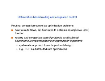
Model definition • We want to describe a network model, with fluctuating numbers of flows • We first need – notation for network structure – abstraction of rate allocation • Then we need to define the random nature of flow arrivals and departures

Network structure (J, R, A) - set of resources J - set of routes R = - if resource j is on route r A 1 jr = - otherwise A 0 jr route resource

Rate allocation - weight of route r w r - number of flows on route r n r - rate of each flow on route r x r = ∈ Given the vector n ( n , r R ) r = ∈ how are the rates x ( x , r R ) r chosen ?

Optimization formulation x = Suppose is chosen to x ( n ) − α 1 x ∑ r w n maximize − α r r 1 r ∑ ≤ ∈ A n x C j J subject to jr r r j r ≥ ∈ x 0 r R r α (weighted -fair allocations, Mo and Walrand 2000) − α 1 x < α < ∞ α = r 0 (replace by if ) log( x ) 1 − α r 1

Solution α 1 / ⎛ ⎞ ⎜ ⎟ = ∑ w ∈ ⎜ ⎟ r x r R r ⎜ ⎟ A p ( n ) jr j ⎝ ⎠ j - shadow price (Lagrange multiplier) p j ( n ) for the resource j capacity constraint Observe alignment with square-root formula when ∑ α = = ≈ 2 2 , w 1 / T , p A p r r r jr j j

α Examples of -fair allocations − α 1 x ∑ maximize r w n − α r r 1 r α 1 / ⎛ ⎞ ⎜ ⎟ ∑ = ∑ w ≤ ∈ ∈ A n x C j J ⎜ ⎟ r x r R subject to jr r r j r ⎜ ⎟ A p ( n ) r jr j ⎝ ⎠ ≥ ∈ j x 0 r R r α → = 0 ( w 1 ) - maximum flow α → = 1 ( w 1 ) - proportionally fair α = = - TCP fair 2 2 ( w 1 / T ) r r - max-min fair α → ∞ = ( w 1 )

= = ∈ n 1 , w 1 r R , r r Example = ∈ C 1 j J j 1/2 1/2 max-min fairness: α → ∞ 1/2 2/3 2/3 proportional fairness: 1/3 α = 1 1 1 maximum flow: 0 α → 0

Flow level model = ∈ Define a Markov process n ( t ) ( n ( t ), r R ) r with transition rates → + ν ∈ at rate n n 1 r R r r r → − μ ∈ at rate n n 1 n x ( n ) r R r r r r r - Poisson arrivals, exponentially distributed file sizes ν - let ρ = μ ∈ r r R , r r the load on route r

Stability? (i.e. positive recurrence?) Suppose vertical streams have priority: then condition for stability is ρ ρ ρ < − ρ − ρ ( 1 ) ( 1 ) 2 1 0 1 2 ρ 0 and not C=1 C=1 ρ < − ρ − ρ min{ 1 , 1 } 0 1 2 (Bonald and Massoulie 2001)

Fairness leads to stability ∑ ρ < ∈ A C j J Suppose jr r j r α and resource allocation is weighted -fair. = ∈ Then the Markov process n ( t ) ( n ( t ), r R ) r is positive recurrent (De Veciana, Lee and Konstantopoulos 1999; Bonald and Massoulie 2001).

Heavy traffic We’re interested in what happens when we approach the edge of the achievable region, when ∑ ρ ≈ ∈ A C j J jr r j r

Balanced fluid model ∑ ρ = ∈ A C j J Suppose jr r j r and consider differential equations d n ( t ) = ν − μ > ∈ r n x ( n ) ( n 0 ) r R r r r r r d t First let’s substitute for the values ∈ of , to give: x r ( n ), r R

α 1 / ⎞ ⎛ ⎜ ⎟ d n ( t ) w = ν − μ ∈ ⎜ ⎟ r r n r R ∑ r r r ⎜ ⎟ d t A p ( n ) jr j ⎝ ⎠ j = n 0 ( care needed when ). r Thus, at an invariant state, α ∑ 1 / ⎛ ⎞ A p ( n ) ⎜ ⎟ ν jr j = ∈ ⎜ j ⎟ r n r R μ r ⎜ ⎟ w r r ⎝ ⎠

State space collapse The following are equivalent: • n is an invariant state • there exists a non-negative vector p with ∑ α 1 / ⎛ ⎞ A p ⎜ ⎟ ν jr j = ∈ j ⎜ ⎟ r n r R μ r ⎜ ⎟ w r r ⎝ ⎠ Thus the set of invariant states forms a J dimensional manifold, parameterized by p .

Workloads n ∑ = r W ( n ) A Let μ j jr r r α = the workload for resource j , and let 1 Define diagonal matrices ρ = ν μ ∈ = ∈ diag ( / , r R ), w diag ( w , r R ) r r r Then W lies in the polyhedral cone − − = μ ρ ≥ 1 1 T { W : W A w A p , p 0 }

Example < α < ∞ 0 μ = = ∈ 1 , w r 1 , r R r ρ + ρ 2 0 slope ρ W 1 = p 0 0 2 ρ 0 slope ρ + ρ 1 0 Each bounding face corresponds to a resource not working at full 2 = capacity p 0 Entrainment : congestion at some resources may prevent other resources from working at their W full capacity. 1

Stationary distribution? W 1 = p p 0 2 2 2 = p 0 W p 1 1 Look for a stationary distribution for W , or equivalently, p. Williams (1987) determined sufficient conditions, in terms of the reflection angles and covariance matrix, for a SRBM in a polyhedral domain to have a product form invariant distribution – a skew symmetry condition

Local traffic condition Assume the matrix A contains the columns of the unit matrix amongst its columns: ⎛ ⎞ . . . . . . . . . . 1 0 0 0 0 ⎜ ⎟ ⎜ ⎟ . . . . . . . . . . 0 1 0 0 0 ⎜ ⎟ = A . . . . . . . . . . 0 0 1 0 0 ⎜ ⎟ ⎜ ⎟ . . . . . . . . . . 0 0 0 1 0 ⎜ ⎟ ⎝ ⎠ . . . . . . . . . . 0 0 0 0 1 i.e. each resource has some local traffic -

Product form under proportional fairness α = = ∈ 1 , w r 1 , r R Under the stationary distribution for the reflected Brownian motion, the (scaled) components of p are independent and exponentially distributed. The corresponding approximation for n is ∑ ≈ ρ ∈ n A p r R r r jr j j where − ∑ ρ ∈ p ~ Exp( C A ) j J j j jr r r Dual random variables are independent and exponential!

Multipath routing ν ν 3 2 C C 3 1 μ ν 1 1 C C 2 3 Routes, as well as flow rates, are chosen μ μ to optimize 3 2 − α 1 x ∑ s w n over source-sink pairs s − α s s 1 s

First cut constraint ν ν 3 2 C C 3 1 μ ν 1 1 C C 2 3 μ ρ + ρ ≤ C + μ C 3 2 1 2 1 2

Second cut constraint ν ν 3 2 C C 3 1 μ ν 1 1 C C 2 3 1 ρ + ρ ≤ C μ μ 1 3 3 3 2 2

Generalized cut constraints In general, stability requires ∑ ρ < ∈ A C j J js j s s - a collection of generalized cut constraints. Provided contains a unit matrix, we again have A the approximation ∑ ≈ ρ ∈ n A p s S js s s j where ∈ j J − ∑ ρ ∈ p ~ Exp( C A ) j J j js j s s Again independent dual random variables, now one for each generalized cut constraint!