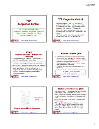
GAIMD Congestion Control Y. Richard Yang and Simon S. Lam, General - PowerPoint PPT Presentation

GAIMD Congestion Control Y. Richard Yang and Simon S. Lam, “General AIMD Congestion Control ” Proceedings IEEE ICNP 2000 Congestion Control, Proceedings IEEE ICNP 2000 , November 2000. GAIMD (Simon S. Lam) 1 3/9/2017 1

Motivation for new congestion control protocols t l t ls  Reducing cwnd to half of its value after a loss g indication is too severe a reduction for some real- time apps (e.g., interactive multimedia)  New apps may use UDP instead of TCP because they do not require reliable delivery  Increasing use of UDP without congestion control would threaten stability of Internet y -> Need new CC protocols for apps that prefer an alternative to TCP alternative to TCP GAIMD (Simon S. Lam) 2 2

TCP-friendly protocols  Alternatives to TCP congestion control with smaller send rate fluctuations  Equati n based rate c ntr l  Equation-based rate control  Datagram Congestion Control Protocol (RFC 4340)  Difficult to measure loss rate and TO in real time  GAIMD in this paper  TCP friendliness to better co exist with TCP  TCP-friendliness to better co-exist with TCP traffic  The send rate of a non-TCP flow should be approximately the same as that of a TCP flow under the same conditions of round-trip time and loss rate GAIMD (Simon S. Lam) 3 3

GAIMD GAIMD  Consider a more general version of AIMD; let α > 0 and 1 > β > 0; let b denote the number of packets acknowledged by each ack k t k l d d b h k α For each new ack received, , ← + W W b bW For a TD ack, ← β W W 1 For a timeout, W ←  Other mechanisms (Slow Start, congestion Oth h i (Sl St t ti indications, and round-trip time estimation) are the same as those of TCP Reno GAIMD (Simon S. Lam) 4 4

Previous models of TCP (f (for α = 1, β = ½) 1 β ½)  No timeout (Matthis et al. 1997)  No timeout (Matthis et al. 1997) 1 3 send rate ( , , ) = = T p RTT b 2 RTT bp p  Timeouts included (Padhye et al. 1998) send rate send rate ( ( , , , ) ) = = T p RTT T b T p RTT T b 0 1 =         2 2 3 3 b bp bp b 2 min 1,3 (1 32 )     + + RTT p p T 0 3 8     GAIMD (Simon S. Lam) 5 5

GAIMD send rate send rate send rate ( ( , , , ) ) = = T T p RTT T b p RTT T b , 0 α β 1 =         2 2 2 (1 ) (1 ) − β − β b p bp 2   min 1,3 (1 32 )   + + RTT p p T   0 (1 ) 2 α + β α      Same model and assumptions as Padhye et al.  p : loss (indication) rate  RTT : mean round-trip time  RTT : mean round-trip time  T 0 : mean timeout value  Reduces to previous formula with α = 1 and β = ½  Send rate decreases with a larger RTT , larger T 0 , or larger b  Send rate increases for a larger α ( > 0), or a larger β  Send rate increases for a larger α ( > 0) or a larger β ( < 1) GAIMD (Simon S. Lam) 6 6

Interpreting the send rate formula  Denominator is sum of the following 2 terms  Denominator is sum of the following 2 terms   2 (1 ) − β b p ( , ( , ) )     = = TD TD p RTT b p RTT b RTT RTT , α β (1 ) α + β   2 ( , , ) (1 32 ) = + TO p T b Q p p T , , 0 0 0 0 α β α β   2 (1 ) − β bp   where min 1,3 = Q   2 α 2 α      Q , probability of a loss indication being a TO, increases towards 1 as p increases increases towards 1 as p increases  For a small p , TD = O(p 0.5 ) >> TO = O(p 1.5 ) but as p increases, the TO term cannot be ignored but s p inc s s th TO t m c nn t b i n d GAIMD (Simon S. Lam) 7 7

Formula validation Formula val dat on  Is the formula accurate? Over what range  Is the formula accurate? Over what range of loss rate p is it accurate?  What is the general trend when the formula loses accuracy? y  When do sending rate variations become W g m significant? GAIMD (Simon S. Lam) 8 8

Simulation setup 16 TCP Reno flows, 16 GAIMD flows, and flows with 16 TCP Reno flows, 16 GAIMD flows, and flows with ON/OFF times to model web-like traffic (UDP flows and short TCP flows) •Mean ON time = 1 s, mean OFF time = 2 s, Pareto distribution •During ON time, each source sends 500 Kbps GAIMD (Simon S. Lam) 9 9

Prediction accuracy  Measure of accuracy:  predicted sending rate/ave. actual sending rate  Validity range of the formula  For each β , vary α from 0.1 to 1.0  For each ( α , β ), vary the number of ON/OFF flows from 10 to 70 to create a loss rate about 1% to 30%  Impact of loss pattern on the accuracy of the formula  Used different kinds of routers: drop-tail and RED GAIMD (Simon S. Lam) 10 10

Accuracy (1) prediction/measurement di ti / t GAIMD (Simon S. Lam) 11 11

Accuracy (2) prediction/measurement prediction/measurement Formula good for loss rate up to 20% up to 20% GAIMD (Simon S. Lam) 12 12

Accuracy (3) prediction/measurement p RED router may not satisfy correlated loss assumption y y p GAIMD (Simon S. Lam) 13 13

Sending Rate Variation (drop-tail) accuracy for individual GAIMD flows and TCP flows accuracy for individual GAIMD flows and TCP flows GAIMD TCP =0.75, drop-tail router α =0.4, =0.4, β =0.75, GAIMD (Simon S. Lam) 14 14

Sending Rate Variation (RED) accuracy for individual GAIMD flows and TCP flows accuracy for individual GAIMD flows and TCP flows TCP GAIMD GAIMD =0.75, RED router E α =0.4, =0.4, β =0.75, GAIMD (Simon S. Lam) 15 15

Summary of Validation Tests  Accurate for loss rate p < 20%  A t f l t 20%  Loss patterns (RED vs drop tail) do not  Loss patterns (RED vs. drop-tail) do not have a large impact on accuracy  Sending rate variance is small for a loss rate of up to 10% p  Trend: rate formulas tend to overestimate when loss rate is high or when α , β are h l h h h aggressive  Overestimates are similar for both TCP and  Overestimates are similar for both TCP and GAIMD (in most experiments) GAIMD (Simon S. Lam) 16 16

TCP-friendly GAIMD  Choose α and β values such that send rate ( , , , ) = T p RTT T b , 0 α β 1 =       2 2 (1 ) (1 ) − β − β b p bp 2   min 1,3 (1 32 )   + + RTT p p T   0 (1 ) 2 α + β α       ( , , , ) = T p RTT T b 1 0 1,2  For all p , only solution is α = 1 and β = 1/2 GAIMD (Simon S. Lam) 17 17

TD TCP-friendly curve ( , , ) ( , , ) = TD p RTT b TD p RTT b , 1 α β 1,2         2 (1 2 (1 ) ) 2 (1 2 (1 1/ 2) 1/ 2) − β β − b b p p b b p p         = RTT RTT (1 ) (1 1/ 2) α + β +     3(1 ) − β = (1 α (1 ) ) + β β GAIMD (Simon S. Lam) 18 18

TO TCP-friendly curve ( , , ) ( , , ) = TO p T b TO p T b , 0 1 0 α β 1,2     2 (1 ) (1 1/ 4) − β − bp bp   2 2 min 1,3 (1 32 ) min 1,3 (1 32 )   + = + p p T p p T   0 0 2 2 α         2 (1 ) 3 − β = = 2 8 α 2 4(1 ) − β α = 3 3 GAIMD (Simon S. Lam) 19 19

Minimizing error over a range of p values 1 , ( ) T p    Error function α β ( ) ( ) 1 β α = − E w p dp ( ) ( ) T T p p 1 0 1,2 where w ( p ) allocates weight p ll t i ht between 0 and 1  For a given β  For a given β , minimize error to get the best α get the best α GAIMD (Simon S. Lam) 20 20

Error as a function of α  β = 0.875 T 0 = 4(RTT)  Optimal value of α increases as threshold increases  Optimal value of α increases as threshold increases GAIMD (Simon S. Lam) 21 21

( α , β ) curves for the three approaches 2 1.8 TD 1.6 TO 1.4 thr=0.1 1 2 1.2 thr=0.2 alpha 1 thr=0.3 0.8 We propose to use p p 0.6 0 6 β =0.875 and α =0.31 0.3125 0.4 0.2 0.2 0 2 0 0.2 0.3 0.4 0.5 0.6 0.7 0.8 beta 0.9 GAIMD (Simon S. Lam) 22 22

Chiu and Jain model Two competing TCP Reno flows:  Additive increase gives slope of 1, as window size increases  Multiplicative decrease reduces window size proportionally equal window size l i d i loss: decrease window by factor of 2 congestion avoidance: additive increase loss: decrease window by factor of 2 congestion avoidance: additive increase congestion avoidance: additive increase Connection 1 window size GAIMD (Simon S. Lam) 23 23

Evolution of Window Sizes  Apply Chiu and Jain [5] model to a TCP flow and a GAIMD flow (no and a GAIMD flow (no timeout, same RTT)  GAIMD with α = 0.31 and β = 0.875 d  Windows of the two flows do not converge flows do not converge to equal window size curve, but zigzag across it it  GAIMD has smaller w ndow s ze window size oscillations GAIMD (Simon S. Lam) 24 24