Conditional Choice Probability Estimators of Single-Agent Dynamic - - PowerPoint PPT Presentation

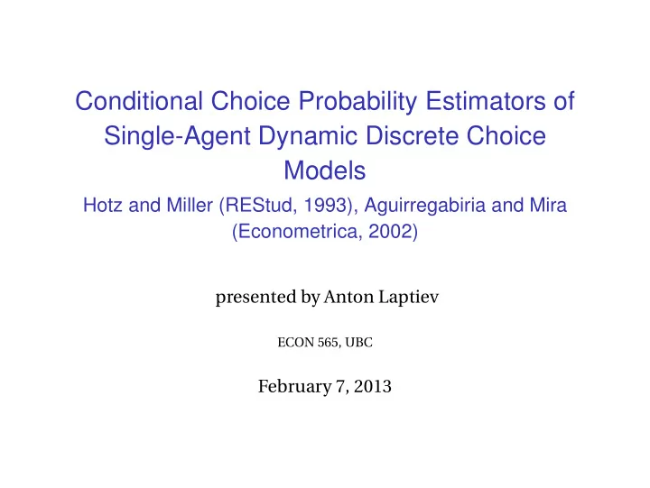
Conditional Choice Probability Estimators of Single-Agent Dynamic Discrete Choice Models

Hotz and Miller (REStud, 1993), Aguirregabiria and Mira (Econometrica, 2002)

presented by Anton Laptiev

ECON 565, UBC

February 7, 2013

Outline

Single-Agent Models Hotz & Miller Estimator Aguirregabiria & Mira Estimator

Single-Agent Models

time is discrete t = 0,1,..,T agents have preferences defined over a sequence of states

• f the world {sit,ait}

sit a vector of state variables that is known at period t ait denotes a decision chosen at t with ait ∈ A = {0,1,...,J}

agents’ preferences are represented by a utility function

T

• j=0

βjU

• ai,t+j, si,t+j
• , β ∈ (0,1)

the optimization problem of an agent

max

a∈A E

• T
• j=0

βjU

• ai,t+j, si,t+j
• | ait, sit

Single-Agent Models

Bellman equation

V(sit) = max

a∈A

• U (a, sit)+β
• V
• si,t+1
• dF
• si,t+1 | a, sit
• choice-specific value function

v(a, sit) ≡ U (a, sit)+β

• V
• si,t+1
• dF
• si,t+1 | a, sit
• the optimal decision rule

α(sit) = arg max

a∈A {v(a, sit)}

assume that sit is divided into two subvectors sit = (xit, ǫit)

Assumptions

Assumption AS

the one-period utility function is additively separable in

• bservable and unobservable components

U (a, xit, ǫit) = u(a, xit)+ǫit (a)

Assumption IID

the unobserved state variables ǫit are identically distributed

• ver agents and over time with cdf Gǫ (ǫit)

Assumption CI

conditional on the current values of the decision and ob-

servable state variables, next period state variables does nor depend on the current ǫ Fx

• xi,t+1 | ait, xit, ǫit
• = Fx
• xi,t+1 | ait, xit

Assumptions

Assumption Logit

the unobserved state variables are independent across al-

ternatives and have an extreme value type I distribution

Assumption DS

the support of xit is discrete and finite

by assumptions IID and CI, the solution to DP problem is

fully characterized by ex ante value function V (xit) =

• V (xit, ǫit) dGǫ (ǫit)

by assumption AS the choice-specific value function can

be written as follows v(a, xit) = u(a, xit)+β

• xi,t+1

V

• xi,t+1
• fx
• xi,t+1 |a, xit
• +ǫit (a)

Forming the Likelihood

Pr

• ait, xit | ˜

ai,t−1, ˜ xi,t−1

• = Pr (ait | xit) fx
• xit | ai,t−1, xi,t−1
• li (θ) =

Ti

• t=1

log P(ait | xit, θ)+

Ti−1

• t=1

log fx

• xi,t+1 | ait, xit, θf
• +log Pr (xi1 | θ)

P(a | x, θ) ≡

• I {α(x, ǫ; θ) = a}dGǫ (ǫ)

=

• v(a, xit)+ǫit (a) > v
• a′, xit
• +ǫit
• a′

∀a′ = a

• dGǫ (ǫit)

The Hotz and Miller Inversion

suppose that payoff function is linear in parameters

u(a, xit; θu) = z(a, xit)′ θu

the choice-specific value function

v(a, xt; θ) = ˜ z(a, xt)θu + ˜ e(a, xt; θ)

˜ z(a, xt; θ) = z(a, xt)+

T−t

• j=1

βj E(xt+j,ǫt+j)|at=a,xt

• z
• α
• xt+j,ǫt+j; θ
• ,xt+j
• = z(a, xt)+

T−t

• j=1

βj Ext+j | at=a,xt

• J
• at+j=0

P

• at+j | xt+j; θ
• z
• at+j, xt+j

The Hotz and Miller Inversion

˜ e(a, xt; θ) =

T−t

• j=1

βj E(xt+j,ǫt+j)|at=a,xt

• ǫ
• α
• xt+j,ǫt+j; θ
• =

T−t

• j=1

βj Ext+j | at=a,xt

• J
• at+j=0

P

• at+j | xt+j; θ
• e
• at+j, xt+j
• e(a, xt) = E
• ǫt(a) | xt, v(a, xt)+ǫt(a) ≥ v(a′, xt)+ǫt(a′) ∀a′ = a
• =

1 P(a | xt)

• ǫt(a)I
• ǫt(a′)−ǫt(a) ≤ v(a, xt)−v(a′, xt) ∀a′ = a
• dGǫ(ǫt)

P(a | xt) =

• ǫt(a)I
• ǫt(a′)−ǫt(a) ≤ v(a, xt)−v(a′, xt) ∀a′ = a
• dGǫ(ǫt)

= ⇒ e(a, xt) = f (P(a | xt), Gǫ, ˜ v(xt)) P(a | xt) = f (Gǫ, ˜ v(xt))

where ˜

v(xt) is a vector of value differences

The Hotz and Miller Inversion

H&M prove that the letter mapping is invertible

= ⇒ e(a, xt) = f (P(a | xt), Gǫ)

by assumption LOGIT, conditional probabilities look as

follows P(a | xt; θ) = exp

• ˜

zˆ

P (a, xt)θu + ˜

eˆ

P (a, xt)

• J

a′=0 exp

• ˜

zˆ

P (a′, xt)θu + ˜

eˆ

P (a′, xt)

• where ˜

zˆ

P and ˜

eˆ

P are defined on all a ∈ A

Example: Renewal Actions

logit errors

V(xt) = log

• a∈A

exp[v(xt, a)]

• +γ

V(xt) = log

• exp
• v(xt, a′)
• a∈A exp[v(xt, a)]

exp[v(xt, a′)]

• +γ

= log

• a∈A

exp

• v(xt, a)−v(xt, a′)
• +v(xt, a′)+γ

= −log

• p(a′ | xt)
• +v(xt, a′)+γ

conditional value function

v(xt, a) = u(xt, a)+β

• v(xt+1,a′)−log
• p(a′|xt+1
• fx(xt+1|xt,a)dxt+1+βγ

Example: Renewal Actions

let a = R indicate the renewal action so that

• fx (xt+1|xt,a)fx (xt+2|xt+1,R)dxt+1 =
• fx
• xt+1|xt,a′

fx (xt+2|xt+1,R)dxt+1 ∀ {a, a′}, xt+2

substitute into the conditional value function

v(xt, a) = u(xt, a)+β

• v(xt+1,R)−log
• p(R|xt+1
• fx(xt+1|xt,a)dxt+1+βγ

= u(xt, a)+β

• u(xt+1,R)−log
• p(R|xt+1
• fx(xt+1|xt,a)dxt+1

+βγ+β2

• V(xt+2) fx (xt+2|xt+1,R)fx (xt+1|xt,a)dxt+2 dxt+1

the last term is constant across all choices made at time t

Estimation

first stage

P(a | xt;) and fx

• xi,t+1 | ait, xit, θf
• are estimated nonpara-

metrically directly from the data

estimate ˜

zˆ

P and ˜

eˆ

P by backward induction (finite T) or us-

ing an iterative procedure (requires stationarity)

second stage

estimate θ by GMM using moment conditions of the form

N

• i=1

Ti

• t=1

H (xit)

• I {ait = a}− ˆ

P(a | xit; θ)

• = 0

Advantages of H&M estimator

computational simplicity relative to full solution

methods

˜

zˆ

P and ˜

eˆ

P are computed only once and remain fixed

during the search for θ

conditional logit assumption along with the assump-

tion of linearity result in the unique solution for the system of GMM equations

pseudo maximum likelihood version of H&M es-

timator is asymptotically equivalent to two-step NFP estimator

Limitations of H&M approach

computational gain relies on (strong) assump-

tions regarding the form of utility function and the structure of unobservable state variables

in finite samples produces larger bias than the

two step NFP estimator (Aguirregabiria & Mira, 2002)

subject to the "curse of dimensionality" cannot accommodate unobserved heterogene-

ity

consistent estimates of conditional choice probabili-

ties cannot be recovered in the first stage

Aguirregabiria & Mira estimator

start from the pseudo likelihood version of H&M estima-

tor Q

• θu, ˆ

P, ˆ θf

• =

N

• i=1

Ti

• t=1

log exp

• ˜

zˆ

P (ait, xit)θu + ˜

eˆ

P (ait, xit)

• J

a′=0 exp

• ˜

zˆ

P (a′, xit)θu + ˜

eˆ

P (a′, xit)

• btain estimates ˆ

θu

compute new estimates of the choice probabilities

ˆ P1 = ˆ P1 (a | x) = exp

• ˜

zˆ

P (a, x)θu + ˜

eˆ

P (a, x)

• J

a′=0 exp

• ˜

zˆ

P (a′, x)θu + ˜

eˆ

P (a′, x)

Aguirregabiria & Mira estimator

given ˆ

P1 one can compute new values ˜ zˆ

P and ˜

eˆ

P

as well as a new pseudo likelihood function Q(·) and maximize it to get a new value of ˆ θu

iterating in this way we can generate a sequence

• f estimators of structural parameters and CCPs

ˆ θu, K, ˆ PK : K = 1,2,...

• : ∀K ≥ 1

ˆ θu,K = arg max

θu∈Θ Q

• θu, ˆ

PK−1, ˆ θf

• ˆ

PK (a | x) = exp

• ˜

zˆ

PK−1 (a, x) ˆ

θu, K + ˜ eˆ

PK−1 (a, x)

• J

a′=0 exp

• ˜

zˆ

PK−1 (a′, x) ˆ

θu, K + ˜ eˆ

PK−1 (a′, x)

Advantages of the Aguirregabiria & Mira estimator

Aguirregabiria & Mira (2002) present Monte Carlo

evidence that iterating in this procedure produces significant reductions in finite sample bias

as K → ∞ the recursive procedure converges to

the two-step NFP estimator even if the initial CCP estimator was inconsistent

A&M show that CCP mapping used in the iter-

ative estimation is a contraction mapping and therefore can be used to compute the solution

• f the DP problem in the space of CCPs