Computer Science & Engineering 423/823 Design and Analysis of - - PowerPoint PPT Presentation

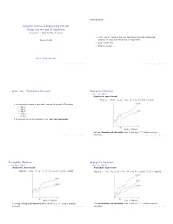
Computer Science & Engineering 423/823 Design and Analysis of Algorithms

Lecture 01 — Shall We Play A Game? Stephen Scott sscott@cse.unl.edu

Introduction

◮ In this course, I assume that you have learned several fundamental

concepts on basic data structures and algorithms

◮ Let’s confirm this ◮ What do I mean ...

... when I say: “Asymptotic Notation”

◮ A convenient means to succinctly express the growth of functions

◮ Big-O ◮ Big-Ω ◮ Big-Θ ◮ Little-o ◮ Little-ω

◮ Important distinctions between these (not interchangeable)

Asymptotic Notation

... when I say: “Big-O”

Asymptotic upper bound O(g(n)) = {f (n) : ∃c, n0 > 0 s.t. ∀n ≥ n0, 0 ≤ f (n) ≤ c g(n)} Can very loosely and informally think of this as a “≤” relation between functions

Asymptotic Notation

... when I say: “Big-Ω”

Asymptotic lower bound Ω(g(n)) = {f (n) : ∃c, n0 > 0 s.t. ∀n ≥ n0, 0 ≤ c g(n) ≤ f (n)} Can very loosely and informally think of this as a “≥” relation between functions

Asymptotic Notation

... when I say: “Big-Θ”

Asymptotic tight bound Θ(g(n)) = {f (n) : ∃c1, c2, n0 > 0 s.t. ∀n ≥ n0, 0 ≤ c1 g(n) ≤ f (n) ≤ c2 g(n)} Can very loosely and informally think of this as a “=” relation between functions

Asymptotic Notation

... when I say: “Little-o”

Upper bound, not asymptotically tight

• (g(n)) = {f (n) : ∀c > 0, ∃n0 > 0 s.t. ∀n ≥ n0, 0 ≤ f (n) < c g(n)}

Upper inequality strict, and holds for all c > 0 Can very loosely and informally think of this as a “<” relation between functions

Asymptotic Notation

... when I say: “Little-ω”

Lower bound, not asymptotically tight ω(g(n)) = {f (n) : ∀c > 0, ∃n0 > 0 s.t. ∀n ≥ n0, 0 ≤ c g(n) < f (n)} f (n) ∈ ω(g(n)) ⇔ g(n) ∈ o(f (n)) Can very loosely and informally think of this as a “>” relation between functions

... when I say: “Upper and Lower Bounds”

◮ Most often, we analyze algorithms and problems in terms of time

complexity (number of operations)

◮ Sometimes we analyze in terms of space complexity (amount of

memory)

◮ Can think of upper and lower bounds of time/space for a specific

algorithm or a general problem

Upper and Lower Bounds

... when I say: “Upper Bound of an Algorithm”

◮ The most common form of analysis ◮ An algorithm A has an upper bound of f (n) for input of size n if there

exists no input of size n such that A requires more than f (n) time

◮ E.g., we know from prior courses that Quicksort and Bubblesort take no

more time than O(n2), while Mergesort has an upper bound of O(n log n)

◮ (But why is Quicksort used more in practice?)

◮ Aside: An algorithm’s lower bound (not typically as interesting) is like a

best-case result

Upper and Lower Bounds

... when I say: “Upper Bound of a Problem”

◮ A problem has an upper bound of f (n) if there exists at least one

algorithm that has an upper bound of f (n)

◮ I.e., there exists an algorithm with time/space complexity of at most f (n)

• n all inputs of size n

◮ E.g., since Mergesort has worst-case time complexity of O(n log n), the

problem of sorting has an upper bound of O(n log n)

◮ Sorting also has an upper bound of O(n2) thanks to Bubblesort and

Quicksort, but this is subsumed by the tighter bound of O(n log n)

Upper and Lower Bounds

... when I say: “Lower Bound of a Problem”

◮ A problem has a lower bound of f (n) if, for any algorithm A to solve

the problem, there exists at least one input of size n that forces A to take at least f (n) time/space

◮ This pathological input depends on the specific algorithm A ◮ E.g., there is an input of size n (reverse order) that forces Bubblesort to

take Ω(n2) steps

◮ Also e.g., there is a different input of size n that forces Mergesort to

take Ω(n log n) steps, but none exists forcing ω(n log n) steps

◮ Since every sorting algorithm has an input of size n forcing Ω(n log n)

steps, the sorting problem has a time complexity lower bound of Ω(n log n)

⇒ Mergesort is asymptotically optimal

Upper and Lower Bounds

... when I say: “Lower Bound of a Problem” (2)

◮ To argue a lower bound for a problem, can use an adversarial argument:

An algorithm that simulates arbitrary algorithm A to build a pathological input

◮ Needs to be in some general (algorithmic) form since the nature of the

pathological input depends on the specific algorithm A

◮ Can also reduce one problem to another to establish lower bounds

◮ Spoiler Alert: This semester we will show that if we can compute convex

hull in o(n log n) time, then we can also sort in time o(n log n); this cannot be true, so convex hull takes time Ω(n log n)

... when I say: “Efficiency”

◮ We say that an algorithm is time- or space-efficient if its worst-case

time (space) complexity is O(nc) for constant c for input size n

◮ I.e., polynomial in the size of the input ◮ Note on input size: We measure the size of the input in terms of the

number of bits needed to represent it

◮ E.g., a graph of n nodes takes O(n log n) bits to represent the nodes and

O(n2 log n) bits to represent the edges

◮ Thus, an algorithm that runs in time O(nc) is efficient ◮ In contrast, a problem that includes as an input a numeric parameter k

(e.g., threshold) only needs O(log k) bits to represent

◮ In this case, an efficient algorithm for this problem must run in time

O(logc k)

◮ If instead polynomial in k, sometimes call this pseudopolynomial

... when I say: “Recurrence Relations”

◮ We know how to analyze non-recursive algorithms to get asymptotic

bounds on run time, but what about recursive ones like Mergesort and Quicksort?

◮ We use a recurrence relation to capture the time complexity and then

bound the relation asymptotically

◮ E.g., Mergesort splits the input array of size n into two sub-arrays,

recursively sorts each, and then merges the two sorted lists into a single, sorted one

◮ If T(n) is time for Mergesort on n elements,

T(n) = 2T(n/2) + O(n)

◮ Still need to get an asymptotic bound on T(n)

Recurrence Relations

... when I say: “Master Theorem” or “Master Method”

◮ Theorem: Let a ≥ 1 and b > 1 be constants, let f (n) be a function,

and let T(n) be defined as T(n) = aT(n/b) + f (n). Then T(n) is bounded as follows:

• 1. If f (n) = O(nlogb a−ǫ) for constant ǫ > 0, then T(n) = Θ(nlogb a)
• 2. If f (n) = Θ(nlogb a), then T(n) = Θ(nlogb a log n)
• 3. If f (n) = Ω(nlogb a+ǫ) for constant ǫ > 0, and if af (n/b) ≤ cf (n) for

constant c < 1 and sufficiently large n, then T(n) = Θ(f (n))

◮ E.g., for Mergesort, can apply theorem with a = b = 2, use case 2, and

get T(n) = Θ

• nlog2 2 log n
• = Θ (n log n)

Recurrence Relations

Other Approaches

Theorem: For recurrences of the form T(αn) + T(βn) + O(n) for α + β < 1, T(n) = O(n) Proof: Top T(n) takes O(n) time (= cn for some constant c). Then calls to T(αn) and T(βn), which take a total of (α + β)cn time, and so on Summing these infinitely yields (since α + β < 1) cn(1 + (α + β) + (α + β)2 + · · · ) = cn 1 − (α + β) = c′n = O(n)

Recurrence Relations

Still Other Approaches

Previous theorem special case of recursion-tree method: (e.g., T(n) = 3T(n/4) + O(n2)) Another approach is substitution method (guess and prove via induction)

Graphs

... when I say: “(Undirected) Graph”

A (simple, or undirected) graph G = (V , E) consists of V , a nonempty set

• f vertices and E a set of unordered pairs of distinct vertices called edges

B D E C A

V={A,B,C,D,E} E={ (A,D),(A,E),(B,D), (B,E),(C,D),(C,E)}

Graphs

... when I say: “Directed Graph”

A directed graph (digraph) G = (V , E) consists of V , a nonempty set of vertices and E a set of ordered pairs of distinct vertices called edges

Graphs

... when I say: “Weighted Graph”

A weighted graph is an undirected or directed graph with the additional property that each edge e has associated with it a real number w(e) called its weight

7 4 3

• 6

3 12

Graphs

... when I say: “Representations of Graphs”

◮ Two common ways of representing a graph: Adjacency list and

adjacency matrix

◮ Let G = (V , E) be a graph with n vertices and m edges

Graphs

... when I say: “Adjacency List”

◮ For each vertex v ∈ V , store a list of vertices adjacent to v ◮ For weighted graphs, add information to each node ◮ How much is space required for storage?

a e b c d a e a d c a c e b c d d b d e c a b c

Graphs

... when I say: “Adjacency Matrix”

◮ Use an n × n matrix M, where M(i, j) = 1 if (i, j) is an edge, 0 otherwise ◮ If G weighted, store weights in the matrix, using ∞ for non-edges ◮ How much is space required for storage?

c e d b a d c b a a b c d e e 0 1 1 1 0 1 0 1 0 1 1 0 0 1 1 1 0 0 0 1 0 1 1 1 0

Algorithmic Techniques

... when I say: “Dynamic Programming”

◮ Dynamic programming is a technique for solving optimization

problems, where we need to choose a “best” solution, as evaluated by an objective function

◮ Key element: Decompose a problem into subproblems, optimally solve

them recursively, and then combine the solutions into a final (optimal) solution

◮ Important component: There are typically an exponential number of

subproblems to solve, but many of them overlap

⇒ Can re-use the solutions rather than re-solving them

◮ Number of distinct subproblems is polynomial ◮ Works for problems that have the optimal substructure property, in

that an optimal solution is made up of optimal solutions to subproblems

◮ Can find optimal solution if we consider all possible subproblems

◮ Example: All-pairs shortest paths

Algorithmic Techniques

... when I say: “Greedy Algorithms”

◮ Another optimization technique ◮ Similar to dynamic programming in that we examine subproblems,

exploiting optimial substructure property

◮ Key difference: In dynamic programming we considered all possible

subproblems

◮ In contrast, a greedy algorithm at each step commits to just one

subproblem, which results in its greedy choice (locally optimal choice)

◮ Examples: Minimum spanning tree, single-source shortest paths

Algorithmic Techniques

... when I say: “Divide and Conquer”

◮ An algorithmic approach (not limited to optimization) that splits a

problem into sub-problems, solves each sub-problem recursively, and then combines the solutions into a final solution

◮ E.g., Mergesort splits input array of size n into two arrays of sizes ⌈n/2⌉

and ⌊n/2⌋, sorts them, and merges the two sorted lists into a single sorted list in O(n) time

◮ Recursion bottoms out for n = 1

◮ Such algorithms often analyzed via recurrence relations

Proof Techniques

... when I say: “Proof by Contradiction”

◮ A proof technique in which we assume the opposite (negation) of the

premise to be proved and then arrive at a contradiction of some other assumption

◮ If we are trying to prove premise P, we assume for sake of contradiction

¬P and conclude something we know is false

◮ If we argue ¬P ⇒ false, then ¬P must be false and P must be true

◮ E.g., to prove there is no greatest even integer:

◮ Assume for sake of contradiction there exists a greatest even integer N

⇒ ∀ even integers n, we have N ≥ n (1)

◮ But M = N + 2 is an even integer since it’s the sum of two even integers,

and M > N

◮ Therefore, our conclusion (1) is false, so our negated premise is false, so

• ur original premise is true

Proof Techniques

... when I say: “Proof by Induction”

◮ A proof technique (typically applied to situations involving non-negative

integers) in which we prove a base case followed by the inductive step

◮ E.g., prove Sn = n i=1 i = n(n + 1)/2

◮ Base case (n = 1): S1 = 1 = n(n + 1)/2 ◮ Inductive step: Assume holds for n and prove it holds for n + 1:

Sn+1 = Sn + (n + 1) = n(n + 1) 2 + (n + 1) = n(n + 1) + 2n + 2 2 = n2 + 3n + 2 2 = (n + 1)(n + 2) 2

◮ Useful for proving invariants in algorithms, where some property always

holds at every step, and therefore at the final step

Proof Techniques

... when I say: “Proof by Construction”

◮ A proof technique often used to prove existence of something by

directly constructing it

◮ E.g., prove that if a < b then there exists a real number c such that

a < c < b

◮ Set c = (a + b)/2 (always exists in R) ◮ Since c − a = (a + b − 2a)/2 = (b − a)/2 > 0 and

b − c = (2b − a − b)/2 = (b − a)/2 > 0, we have constructed a c such that a < c < b

◮ We will use this extensively when we study NP-completeness

Proof Techniques

... when I say: “Proof by Contrapositive”

◮ Recall that P ⇒ Q is logically equivalent to ¬Q ⇒ ¬P via

contraposition (compare truth tables to convince yourself)

◮ E.g., prove that if x2 is even, then x is even

◮ Contrapositive says: If x is not even, then x2 is not even ◮ This is easily shown true since x is odd, and the product of two odd

numbers is odd

◮ Since contrapositive is true, original premise is true

◮ Very helpful when proving P ⇔ Q (“P if and only if Q”) since we could

prove:

◮ P ⇒ Q and ¬P ⇒ ¬Q OR ◮ P ⇒ Q and Q ⇒ P (often simpler)

◮ We will use this extensively when we study NP-completeness

Conclusion

◮ This was a deliberately brief overview of concepts you should already

know

◮ I expect you to understand it well during lectures, homeworks, and exams ◮ It is all covered in depth in the textbook and other resources!