Computational Logic Fundamentals of Definite Programs: Syntax and - PowerPoint PPT Presentation
Computational Logic Fundamentals of Definite Programs: Syntax and Semantics 1 Towards Logic Programming Conclusion: resolution is a complete and effective deduction mechanism using: Horn clauses (related to D efinite programs), L
Computational Logic Fundamentals of Definite Programs: Syntax and Semantics 1
Towards Logic Programming • Conclusion: resolution is a complete and effective deduction mechanism using: Horn clauses (related to “ D efinite programs”), L inear, Input strategy Breadth-first exploration of the tree (or an equivalent approach) (possibly ordered clauses, but not required – see S election rule later) • Very close to what is generally referred to as SLD-resolution (see later) • This allows to some extent realizing Greene’s dream (within the theoretical limits of the formal method), and efficiently! 2
Towards Logic Programming (Contd.) • Given these results, why not use logic as a general purpose programming language ? [Kowalski 74] • A “logic program” would have two interpretations: ⋄ Declarative (“LOGIC”): the logical reading (facts, statements, knowledge) ⋄ Procedural (“CONTROL ”): what resolution does with the program • ALGORITHM = LOGIC + CONTROL • Specify these components separately • Often, worrying about control is not needed at all (thanks to resolution) • Control can be effectively provided through the ordering of the literals in the clauses 3
Towards Logic Programming: Another (more compact) Clausal Form • All formulas are transformed into a set of Clauses . ⋄ A clause has the form: conc 1 , ..., conc m ← cond 1 , ..., cond n where conc 1 , ..., conc m cond 1 , ..., cond n � �� � � �� � “or” “and” are literals, and are the conclusions and conditions of a rule: conc 1 , ..., conc m ← cond 1 , ..., cond n � �� � � �� � “conclusions” “conditions” ⋄ All variables are implicitly universally quantified: (if X 1 , ..., X k are the variables) ∀ X 1 , ..., X k conc 1 ∨ ... ∨ conc m ← cond 1 ∧ ... ∧ cond n • More compact than the traditional clausal form: ⋄ no connectives, just commas ⋄ no need to repeat negations: all negated atoms on one side, non-negated ones on the other • A Horn Clause then has the form: conc 1 ← cond 1 , ..., cond n where n can be zero and possibly conc 1 empty. 4
Some Logic Programming Terminology – “Syntax” of Logic Programs • Definite Program: a set of positive Horn clauses head ← goal 1 , ..., goal n • The single conclusion is called the head . • The conditions are called “goals” or “procedure calls”. • goal 1 ,...,goal n ( n ≥ 0 ) is called the “body”. • if n = 0 the clause is called a “fact” (and the arrow is normally deleted) • Otherwise it is called a “rule” • Query (question): a negative Horn clause (a “headless” clause) • A procedure is a set of rules and facts in which the heads have the same predicate symbol and arity. • Terms in a goal are also called “arguments”. 5
Some Logic Programming Terminology (Contd.) • Examples: grandfather(X,Y) ← father (X,Z), mother(Z,Y). grandfather(X,Y) ← . grandfather(X,Y). ← grandfather(X,Y). 6
LOGIC: Declarative “Reading” (Informal Semantics) • A rule (has head and body) head ← goal 1 , ..., goal n . which contains variables X 1 , ..., X k can be read as for all X 1 , ..., X k : “head” is true if “goal 1 ” and ... and “goal n ” are true • A fact n=0 (has only head) head. for all X 1 , ..., X k : “head” is true (always) • A query (the headless clause) ← goal 1 , ..., goal n can be read as: for which X 1 , ..., X k are “goal 1 ” and ... and “goal n ” true? 7
LOGIC: Declarative Semantics – Herbrand Base and Universe • Given a first-order language L , with a non-empty set of variables, constants, function symbols, relation symbols, connectives, quantifiers, etc. and given a syntactic object A , ground ( A ) = { Aθ |∃ θ ∈ Subst, var ( Aθ ) = ∅} i.e. the set of all “ground instances” of A . • Given L , U L (Herbrand universe) is the set of all ground terms of L . • B L (Herbrand Base) is the set of all ground atoms of L . • Similarly, for the language L P associated with a given program P we define U P , and B P . • Example: P = { p ( f ( X )) ← p ( X ) . p ( a ) . q ( a ) . q ( b ) . } U P = { a, b, f ( a ) , f ( b ) , f ( f ( a )) , f ( f ( b )) , . . . } B P = { p ( a ) , p ( b ) , q ( a ) , q ( b ) , p ( f ( a )) , p ( f ( b )) , q ( f ( a )) , . . . } 8
Herbrand Interpretations and Models • A Herbrand Interpretation is a subset of B L , i.e. the set of all Herbrand interpretations I L = ℘ ( B L ) . (Note that I L forms a complete lattice under ⊆ – important for fixpoint operations to be introduced later). • Example: P = { p ( f ( X )) ← p ( X ) . p ( a ) . q ( a ) . q ( b ) . } U P = { a, b, f ( a ) , f ( b ) , f ( f ( a )) , f ( f ( b )) , . . . } B P = { p ( a ) , p ( b ) , q ( a ) , q ( b ) , p ( f ( a )) , p ( f ( b )) , q ( f ( a )) , . . . } I P = all subsets of B P • A Herbrand Model is a Herbrand interpretation which contains all logical consequences of the program. • The Minimal Herbrand Model H P is the smallest Herbrand interpretation which contains all logical consequences of the program. (It is unique.) • Example: H P = { q ( a ) , q ( b ) , p ( a ) , p ( f ( a )) , p ( f ( f ( a ))) , . . . } 9
Declarative Semantics, Completeness, Correctness • Declarative semantics of a logic program P : the set of ground facts which are logical consequences of the program (i.e., H P ). (Also called the “least model” semantics of P ). • Intended meaning of a logic program P : the set M of ground facts that the user expects to be logical consequences of the program. • A logic program is correct if H P ⊆ M . • A logic program is complete if M ⊆ H P . • Example: father(john,peter). father(john,mary). mother(mary,mike). grandfather(X,Y) ← father(X,Z), father(Z,Y). with the usual intended meaning is correct but incomplete . 10
CONTROL: Linear (Input) Resolution in this Clausal Form We now turn to the operational semantics of logic programs, given by a concrete operational procedure: Linear (Input) Resolution . • Complementary literals: ⋄ in two different clauses ⋄ on different sides of ← ⋄ unifiable with unifier θ father(john,mary) ← grandfather(X,Y) ← father(X,Z) , mother(Z,Y) θ = { X/john, Z/mary } 11
CONTROL: Linear (Input) Resolution in this Clausal Form (Contd.) • Resolution step (linear, input, ...): ⋄ given a clause and a resolvent, we can build a new resolvent which follows from them by: * renaming apart the clause (“standardization apart” step) * putting all the conclusions to the left of the ← * putting all the conditions to the right of the ← * if there are complementary literals (unifying literals at different sides of the arrow in the two clauses), eliminating them and applying θ to the new resolvent • LD-Resolution: linear (and input) resolution, applied to definite programs Note that then all resolvents are negative Horn clauses (like the query). 12
Example • from father(john,peter) ← mother(mary,david) ← we can infer father(john,peter), mother(mary,david) ← • from father(john,mary) ← grandfather(X,Y) ← father(X,Z), mother(Z,Y) we can infer grandfather(john,Y’) ← mother(mary,Y’) 13
CONTROL: A proof using LD-Resolution • Prove “grandfather(john,david) ← ” using the set of axioms: 1. father(john,peter) ← 2. father(john,mary) ← 3. father(peter,mike) ← 4. mother(mary,david) ← 5. grandfather(L,M) ← father (L,N), father(N,M) 6. grandfather(X,Y) ← father (X,Z), mother(Z,Y) • We introduce the predicate to prove (negated!) 7. ← grandfather(john,david) • We start resolution: e.g. 6 and 7 8. ← father(john,Z 1 ), mother(Z 1 ,david) X 1 /john, Y 1 /david • using 2 and 8 Z 1 /mary 9. ← mother(mary,david) • using 4 and 9 ← 14
CONTROL: Rules and SLD-Resolution • Two control-related issues are still left open in LD-resolution. Given a current resolvent R and a set of clauses K : ⋄ given a clause C in K , several of the literals in R may unify the non-negated a complementary literal in C ⋄ given a literal L in R , it may unify with complementary literals in several clauses in K • A Computation (or Selection rule) is a function which, given a resolvent (and possibly the proof tree up to that point) returns (selects) a literal from it. This is the goal that will be used next in the resolution process. • A Search rule is a function which, given a literal and a set of clauses (and possibly the proof tree up to that point), returns a clause from the set. This is the clause that will be used next in the resolution process. 15
CONTROL: Rules and SLD-Resolution (Contd.) • SLD-resolution: Linear resolution for Definite programs with Selection rule. • An SLD-resolution method is given by the combination of a computation (or selection) rule and a search rule . • Independence of the computation rule : Completeness does not depend on the choice of the computation rule. • Example: a “left-to-right” rule (as in ordered resolution) does not impair completeness – this coincides with the completeness result for ordered resolution. • Fundamental result: “Declarative” semantics ( H P ) ≡ “operational” semantics (SLD-resolution) I.e., all the facts in H P can be deduced using SLD-resolution. 16
Recommend

More recommend
Explore More Topics
Stay informed with curated content and fresh updates.