Comparison of Local Feature Descriptors Subhransu Maji Department - PowerPoint PPT Presentation
Outline Introduction Benchmarks Experiments and Results Future Work Comparison of Local Feature Descriptors Subhransu Maji Department of EECS, University of California, Berkeley. December 13, 2006 Subhransu Maji Comparison of Local
Outline Introduction Benchmarks Experiments and Results Future Work Comparison of Local Feature Descriptors Subhransu Maji Department of EECS, University of California, Berkeley. December 13, 2006 Subhransu Maji Comparison of Local Feature Descriptors
Outline Introduction Benchmarks Experiments and Results Future Work Introduction 1 Local Features Benchmarks 2 Mikolajczyk’s Dataset Caltech 101 Dataset Experiments and Results 3 Evaluation of Feature Detectors Evaluation of Feature Descriptors Future Work 4 Subhransu Maji Comparison of Local Feature Descriptors
Outline Introduction Benchmarks Local Features Experiments and Results Future Work Applications of Local Features Multi Camera Scene reconstruction. Robust to Backgrounds, Occlusions Compact Representation of Objects for Matching, Recognition and Tracking. Lots of uses, Lots of options. This work tries to address the issue of what features are suitable for what task, which is currently a black art!! Subhransu Maji Comparison of Local Feature Descriptors
Outline Introduction Benchmarks Local Features Experiments and Results Future Work Key properties of a good local feature Must be highly distinctive, i.e. low probability of a mismatch. Should be easy to extract. Invariance, a good local feature should be tolerant to. Image noise Changes in illumination Uniform scaling Rotation Minor changes in viewing direction Question: How to construct the local feature to achieve invariance to the above? Subhransu Maji Comparison of Local Feature Descriptors
Outline Introduction Benchmarks Local Features Experiments and Results Future Work Various Feature Detectors Harris detector find points at a fixed scale. Harris Laplace detector uses the scale-adapted Harris function to localize points in scale-space. It then selects the points for which the Laplacian-of-Gaussian attains a maximum over scale. Hessian Laplace localizes points in space at the local maxima of the Hessian determinant and in scale at the local maxima of the Laplacian-of-Gaussian. Harris/Hessian Affine detector does an affine adaptation of the Harris/Hessian Laplace using the second moment matrix. Maximally Stable Exremal Regions detector finds regions such that pixels inside the MSER have either higher (bright extremal regions) or lower (dark extremal regions) intensity than all the pixels on its outer boundary. Uniform Detector (unif) - Select 500 points uniformly on the edge maps by rejection sampling. Subhransu Maji Comparison of Local Feature Descriptors
Outline Introduction Benchmarks Local Features Experiments and Results Future Work Various Feature Descriptors Scale Invariant Feature Transformation A local image is path is divided into a grid (typically 4x4) and a orientation histogram is computed for each of these cells. Shape Contexts computes the ditance and orientaion histogram of other points relative to the interst point. Image Moments These compute the descriptors by taking various higher order image moments. Jet Decriptors These are essentially higher order derivatives of the image at the interest point Gradient Location and Orientaiton Histogram As the name suggests it constructs a feature out of the image using the Histogram of location and Orientation in of points in a window around the interest point. Geometric Blur These compute the average of the edge signal response over small tranformations. Tunable parameters include the blur gradient( β = 1), base blur ( α = 0 . 5) and scale multiplier ( s = 9). Subhransu Maji Comparison of Local Feature Descriptors
Outline Introduction Benchmarks Local Features Experiments and Results Future Work Example Detections Subhransu Maji Comparison of Local Feature Descriptors
Outline Introduction Mikolajczyk’s Dataset Benchmarks Caltech 101 Dataset Experiments and Results Future Work Evaluation Criteria We want the feature to be repeatable, correct − matches repeatability = ground − truth − matches Descriptor Performance: recall vs 1-precision graphs. recall = # correct matches # correspondances correct matches found by neareast neignbour matching in the feature space. correspondances obtained from ground truth matching. # falsematches 1 − precision = # false matches +# correct matces Subhransu Maji Comparison of Local Feature Descriptors
Outline Introduction Mikolajczyk’s Dataset Benchmarks Caltech 101 Dataset Experiments and Results Future Work Mikolajczyk’s Dataset 8 Datasets, 6 Images per dataset. Ground Truth Homography available for these Images. Subhransu Maji Comparison of Local Feature Descriptors
Outline Introduction Mikolajczyk’s Dataset Benchmarks Caltech 101 Dataset Experiments and Results Future Work Caltech 101 Dataset 101 Categories, man-made objects, motifs, animals and plants. Foreground Mask is available. Obtain ground truth based on a rough alignement of the contours. Determine the scale, translation which maximizes area overlap of the contours. Correspondance: Features of the images within a threshold distance(10 Pixels) under the transformation. Many clasification techniques use the structure of image for computing similarity. For e.g. SC based caracter recognition using TSP. The performance of these algorithms is dependent on detecting features on the right positions. Ideally we would want the descriptor performance to be better on such a softer notion of matching. Subhransu Maji Comparison of Local Feature Descriptors
Outline Introduction Mikolajczyk’s Dataset Benchmarks Caltech 101 Dataset Experiments and Results Future Work Best 8 and Worst 8 0 0 50 50 40 50 50 50 60 100 100 80 100 100 100 100 40 150 150 150 120 150 150 60 140 200 200 80 80 200 200 160 200 90 100 180 100 250 250 250 110 250 250 200 120 120 220 300 130 300 140 300 50 100 150 200 250 300 100 150 200 300 350 400 50 100 150 200 250 0 50 100 150 200 250 40 60 80 100 120 140 160 180 200 220 50 100 150 200 250 300 40 60 80 100 120 140 160 180 200 220 240 0.9781 0.9717 0.9642 0.9490 0.9486 0.9483 0.9405 0.9223 0 60 50 20 50 40 80 20 100 60 100 40 100 80 100 120 60 150 80 100 120 150 140 100 120 140 20 160 200 120 40 140 160 200 180 140 60 60 160 180 80 200 250 160 80 180 200 180 100 100 250 200 220 220 200 120 0 50 100 150 200 250 300 0 20 40 60 80 100 120 140 160 180 100 150 200 250 50 100 150 200 250 100 120 140 160 180 200 220 50 100 150 200 250 50 100 150 200 250 300 50 100 150 200 250 300 0.7097 0.6934 0.6919 0.6658 0.6614 0.6444 0.6426 0.3318 Subhransu Maji Comparison of Local Feature Descriptors
Outline Introduction Mikolajczyk’s Dataset Benchmarks Caltech 101 Dataset Experiments and Results Future Work Example Ground Truth Matches 50 50 100 150 100 200 150 250 300 100 200 300 400 500 600 350 100 200 300 400 500 600 700 800 900 1000 Faces car side 50 100 50 150 200 100 250 150 50 100 150 200 250 300 350 400 450 500 100 200 300 400 500 600 stop sign Motorbikes Figure: Ground Truth matches. We use the harris Affine detector with a distance threshold of 5 pixels Subhransu Maji Comparison of Local Feature Descriptors
Outline Introduction Evaluation of Feature Detectors Benchmarks Evaluation of Feature Descriptors Experiments and Results Future Work Repeatability Results on Benchmarks Mikolajczyk Dataset: MSER was generally the best followed by Hessian Affine. Hessian-Affine and Harris-Affine provide more regions than the other detectors, which is useful in matching scenes with occlusion and clutter. Caltech 101 Dataset: Hessian Affine, Hessian Laplace, MSER, UNIF all perform equally well. Hessian Affine is slightly better than others in most cases. Almost any detector is equally good as the matching is softer. Subhransu Maji Comparison of Local Feature Descriptors
Outline Introduction Evaluation of Feature Detectors Benchmarks Evaluation of Feature Descriptors Experiments and Results Future Work Desciptor Performance on Mikolajczyk’s Dataset Effect of scale − bikes Effect of scale − trees 0.9 0.7 gb gb sift sift sc sc 0.8 spin spin 0.6 mom mom jla jla 0.7 0.5 0.6 frac of correct frac of correct 0.4 0.5 0.4 0.3 0.3 0.2 0.2 0.1 0.1 0 0 0 0.1 0.2 0.3 0.4 0.5 0.6 0.7 0.8 0.9 1 0 0.1 0.2 0.3 0.4 0.5 0.6 0.7 0.8 0.9 1 1−precision 1−precision (1)bikes (2)trees Effect of scale − graf Effect of scale − wall 0.45 0.45 gb gb sift sift sc sc 0.4 0.4 spin spin mom mom jla jla 0.35 0.35 0.3 0.3 frac of correct frac of correct 0.25 0.25 0.2 0.2 0.15 0.15 0.1 0.1 0.05 0.05 0 0 0 0.1 0.2 0.3 0.4 0.5 0.6 0.7 0.8 0.9 1 0 0.1 0.2 0.3 0.4 0.5 0.6 0.7 0.8 0.9 1 1−precision 1−precision (3)graffiti (4)wall Subhransu Maji Comparison of Local Feature Descriptors
Recommend
More recommend
Explore More Topics
Stay informed with curated content and fresh updates.
