6.869 Advances in Computer Vision Prof. Bill Freeman March 3, 2005 - PowerPoint PPT Presentation

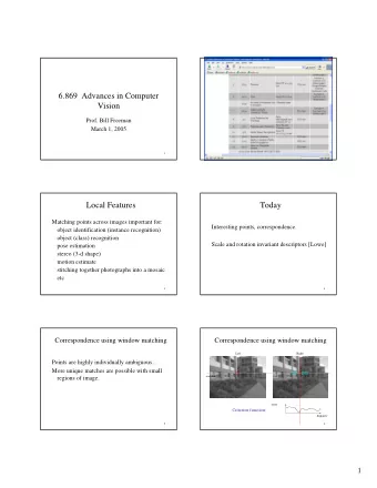
6.869 Advances in Computer Vision Prof. Bill Freeman March 3, 2005 Image and shape descriptors – Affine invariant features – Comparison of feature descriptors – Shape context Readings: Mikolajczyk and Schmid; Belongie et al

Matching with Invariant Features Darya Frolova, Denis Simakov The Weizmann Institute of Science March 2004 http://www.wisdom.weizmann.ac.il/~deniss/vision_spring04/files/InvariantFeatures.ppt

Example: Build a Panorama M. Brown and D. G. Lowe. Recognising Panoramas. ICCV 2003

How do we build panorama? • We need to match (align) images

Matching with Features •Detect feature points in both images

Matching with Features •Detect feature points in both images •Find corresponding pairs

Matching with Features •Detect feature points in both images •Find corresponding pairs •Use these pairs to align images

Matching with Features • Problem 1: – Detect the same point independently in both images no chance to match! We need a repeatable detector

Matching with Features • Problem 2: – For each point correctly recognize the corresponding one ? We need a reliable and distinctive descriptor

More motivation… • Feature points are used also for: – Image alignment (homography, fundamental matrix) – 3D reconstruction – Motion tracking – Object recognition – Indexing and database retrieval – Robot navigation – … other

Contents • Harris Corner Detector – Description – Analysis • Detectors – Rotation invariant – Scale invariant – Affine invariant • Descriptors – Rotation invariant – Scale invariant – Affine invariant

An introductory example: Harris corner detector C.Harris, M.Stephens. “A Combined Corner and Edge Detector”. 1988

The Basic Idea • We should easily recognize the point by looking through a small window • Shifting a window in any direction should give a large change in intensity

Harris Detector: Basic Idea “flat” region: “edge”: “corner”: no change in no change along significant change all directions the edge direction in all directions

Contents • Harris Corner Detector – Description – Analysis • Detectors – Rotation invariant – Scale invariant – Affine invariant • Descriptors – Rotation invariant – Scale invariant – Affine invariant

Harris Detector: Mathematics Change of intensity for the shift [ u,v ]: [ ] ∑ 2 = + + − E u v ( , ) w x y ( , ) I x ( u y , v ) I x y ( , ) x y , Window Shifted Intensity function intensity Window function w(x,y) = or 1 in window, 0 outside Gaussian

Harris Detector: Mathematics For small shifts [ u,v ] we have a bilinear approximation: ⎡ ⎤ u [ ] ≅ E u v ( , ) u v , M ⎢ ⎥ ⎣ ⎦ v where M is a 2 × 2 matrix computed from image derivatives: ⎡ ⎤ 2 I I I ∑ = x x y ⎢ ⎥ M w x y ( , ) 2 ⎢ ⎥ I I I ⎣ ⎦ x y , x y y

Harris Detector: Mathematics Intensity change in shifting window: eigenvalue analysis ⎡ ⎤ u [ ] λ 1 , λ 2 – eigenvalues of M ≅ E u v ( , ) u v , M ⎢ ⎥ ⎣ ⎦ v direction of the fastest change Ellipse E(u,v) = const direction of the slowest change ( λ max ) -1/2 ( λ min ) -1/2

Harris Detector: Mathematics λ 2 Classification of “Edge” λ 2 >> λ 1 image points using “Corner” eigenvalues of M : λ 1 and λ 2 are large, λ 1 ~ λ 2 ; E increases in all directions λ 1 and λ 2 are small; “Edge” E is almost constant “Flat” λ 1 >> λ 2 in all directions region λ 1

Harris Detector: Mathematics Measure of corner response: ( ) 2 = − R det M k trace M = λ λ det M 1 2 = λ + λ trace M 1 2 ( k – empirical constant, k = 0.04-0.06)

cf David Lowe’s analysis

Harris Detector: Mathematics λ 2 “Edge” “Corner” • R depends only on R < 0 eigenvalues of M • R is large for a corner R > 0 • R is negative with large magnitude for an edge • | R | is small for a flat region “Flat” “Edge” |R| small R < 0 λ 1

Harris Detector • The Algorithm: – Find points with large corner response function R ( R > threshold) – Take the points of local maxima of R

Harris Detector: Workflow

Harris Detector: Workflow Compute corner response R

Harris Detector: Workflow Find points with large corner response: R> threshold

Harris Detector: Workflow Take only the points of local maxima of R

Harris Detector: Workflow

Harris Detector: Summary • Average intensity change in direction [ u,v ] can be expressed as a bilinear form: ⎡ ⎤ u [ ] ≅ E u v ( , ) u v , M ⎢ ⎥ ⎣ ⎦ v • Describe a point in terms of eigenvalues of M : measure of corner response ( ) 2 = λ λ − λ + λ R k 1 2 1 2 • A good (corner) point should have a large intensity change in all directions , i.e. R should be large positive

Contents • Harris Corner Detector – Description – Analysis • Detectors – Rotation invariant – Scale invariant – Affine invariant • Descriptors – Rotation invariant – Scale invariant – Affine invariant

Harris Detector: Some Properties • Rotation invariance Ellipse rotates but its shape (i.e. eigenvalues) remains the same Corner response R is invariant to image rotation

Harris Detector: Some Properties • Partial invariance to affine intensity change � Only derivatives are used => invariance to intensity shift I → I + b � Intensity scale: I → a I R R threshold x (image coordinate) x (image coordinate)

Harris Detector: Some Properties • But: non-invariant to image scale ! All points will be Corner ! classified as edges

Harris Detector: Some Properties • Quality of Harris detector for different scale changes Repeatability rate: # correspondences # possible correspondences C.Schmid et.al. “Evaluation of Interest Point Detectors”. IJCV 2000

Contents • Harris Corner Detector – Description – Analysis • Detectors – Rotation invariant – Scale invariant – Affine invariant • Descriptors – Rotation invariant – Scale invariant – Affine invariant

We want to: detect the same interest points regardless of image changes

Models of Image Change • Geometry – Rotation – Similarity (rotation + uniform scale) – Affine (scale dependent on direction) valid for: orthographic camera, locally planar object • Photometry – Affine intensity change ( I → a I + b )

Contents • Harris Corner Detector – Description – Analysis • Detectors – Rotation invariant – Scale invariant – Affine invariant • Descriptors – Rotation invariant – Scale invariant – Affine invariant

Rotation Invariant Detection • Harris Corner Detector C.Schmid et.al. “Evaluation of Interest Point Detectors”. IJCV 2000

Contents • Harris Corner Detector – Description – Analysis • Detectors – Rotation invariant – Scale invariant – Affine invariant • Descriptors – Rotation invariant – Scale invariant – Affine invariant

Scale Invariant Detection • Consider regions (e.g. circles) of different sizes around a point • Regions of corresponding sizes will look the same in both images

Scale Invariant Detection • The problem: how do we choose corresponding circles independently in each image?

Scale Invariant Detection • Solution: – Design a function on the region (circle), which is “scale invariant” (the same for corresponding regions, even if they are at different scales) Example : average intensity. For corresponding regions (even of different sizes) it will be the same. – For a point in one image, we can consider it as a function of region size (circle radius) Image 1 f f Image 2 scale = 1/2 region size region size

Scale Invariant Detection • Common approach: Take a local maximum of this function Observation : region size, for which the maximum is achieved, should be invariant to image scale. Important: this scale invariant region size is found in each image independently! Image 1 f f Image 2 scale = 1/2 s 1 s 2 region size region size

Scale Invariant Detection • A “good” function for scale detection: has one stable sharp peak f f f Good ! bad bad region size region size region size • For usual images: a good function would be a one which responds to contrast (sharp local intensity change)

Scale Invariant Detection f = ∗ Kernel Image • Functions for determining scale Kernels: ( ) = σ σ + σ 2 L G ( , , x y ) G ( , , x y ) xx yy (Laplacian) = σ − σ DoG G x y k ( , , ) G x y ( , , ) (Difference of Gaussians) where Gaussian 2 + 2 x y − Note: both kernels are invariant to σ = σ 2 G x y ( , , ) 1 e 2 scale and rotation πσ 2

Scale Invariant Detection • Compare to human vision: eye’s response Shimon Ullman, Introduction to Computer and Human Vision Course, Fall 2003