Commuting, Migration, and Local Employment Elasticities Ferdinando - PDF document
Commuting, Migration, and Local Employment Elasticities Ferdinando Monte Georgetown University Stephen Redding Princeton University Esteban Rossi-Hansberg Princeton University October 2017 Monte, Redding, Rossi-Hansberg Local Employment
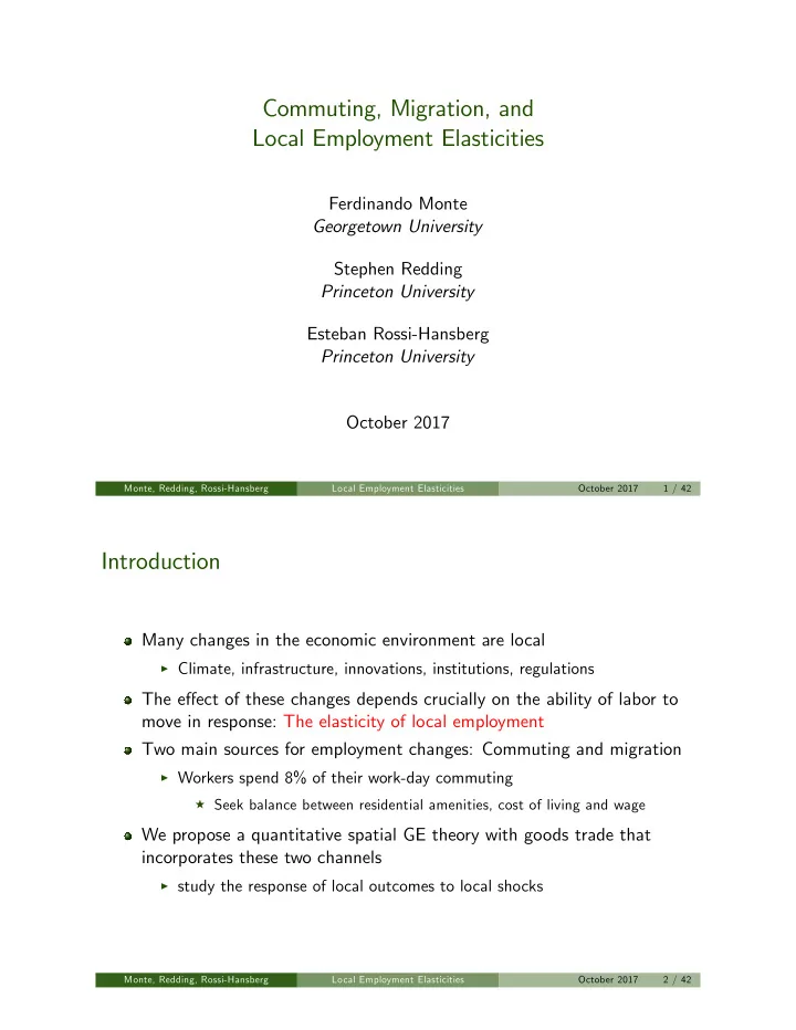
Commuting, Migration, and Local Employment Elasticities Ferdinando Monte Georgetown University Stephen Redding Princeton University Esteban Rossi-Hansberg Princeton University October 2017 Monte, Redding, Rossi-Hansberg Local Employment Elasticities () October 2017 1 / 42 Introduction Many changes in the economic environment are local I Climate, infrastructure, innovations, institutions, regulations The e§ect of these changes depends crucially on the ability of labor to move in response: The elasticity of local employment Two main sources for employment changes: Commuting and migration I Workers spend 8% of their work-day commuting F Seek balance between residential amenities, cost of living and wage We propose a quantitative spatial GE theory with goods trade that incorporates these two channels I study the response of local outcomes to local shocks Monte, Redding, Rossi-Hansberg Local Employment Elasticities () October 2017 2 / 42
Introduction We discipline our quantitative model to match I Gravity in goods trade I Gravity in commuting áows I Distribution of employment, residents and wages across counties The quantitative importance of these two channels varies across counties depending on their local characteristics I Leads to signiÖcant heterogeneity in the employment elasticity I Locations are not independent spatial units as often assumed in cross-section regressions I Underscores general equilibrium e§ects A§ects the estimated e§ects of most local policies and shocks and their external validity I Heterogeneity is well accounted for by commuting links Provide empirical evidence for the importance of commuting I Shift-share analysis, Million Dollar Plants, China Shock Monte, Redding, Rossi-Hansberg Local Employment Elasticities () October 2017 3 / 42 Key Mechanisms Productivity di§erences and home market e§ects I Forces for the concentration of economic activity Inelastic housing supply and heterogeneous preferences I Forces for the dispersion of economic activity Commuting allows workers to access high productivity locations without having to live there I E§ectively reduces the congestion e§ect in high productivity areas Elasticity of employment with respect to local shocks (e.g. productivity, amenities, infrastructure) depends on I Ability to attract migrants I Ability to attract commuters from surrounding locations Monte, Redding, Rossi-Hansberg Local Employment Elasticities () October 2017 4 / 42
The Extent of Commuting Counties become more open over time .1 Density .05 0 0 .2 .4 .6 .8 1 Share of Residents that Work in the County Where They Live 1960 1970 1980 1990 2000 Commuting links are sizeable and heterogeneous Min p5 p10 p25 p50 p75 p90 p95 Max Mean Commuters from Residence County 0.00 0.03 0.06 0.14 0.27 0.42 0.53 0.59 0.82 0.29 Commuters to Workplace County 0.00 0.03 0.07 0.14 0.20 0.28 0.37 0.43 0.81 0.22 County Employment/Residents 0.26 0.60 0.67 0.79 0.92 1.02 1.11 1.18 3.88 0.91 Commuters from Residence CZ 0.00 0.00 0.01 0.03 0.07 0.12 0.18 0.22 0.49 0.08 Commuters to Workplace CZ 0.00 0.00 0.01 0.03 0.07 0.10 0.13 0.15 0.25 0.07 CZ Employment/Residents 0.63 0.87 0.91 0.97 1.00 1.01 1.03 1.04 1.12 0.98 Tabulations on 3,111 counties and 709 CZ after eliminating business trips (trips longer than 120km). Weighted Table Monte, Redding, Rossi-Hansberg Local Employment Elasticities () October 2017 5 / 42 Related Literature Quantitative international trade literature on costly trade in goods I Eaton and Kortum (2002) and extensions Economic geography literature on goods trade and factor mobility I Krugman (1991), Fujita et al. (1999), Rossi-Hansberg (2005), Allen and Arkolakis (2014), Allen et al. (2015), Caliendo et al. (2014), Desmet and Rossi-Hansberg (2014), Redding (2014) Urban literature on costly trade in people (commuting) I Alonso (1964), Mills (1967), Muth (1969), Lucas and Rossi-Hansberg (2002), Desmet and Rossi-Hansberg (2013), Ahlfeldt et al. (2014), Behrens et al. (2014), Monte (2016) Local labor markets literature I Greenstone et al. (2010), Moretti (2011), Busso et al. (2013), Autor et al. (2013), Diamond (2013), Notowidigdo (2013), Yagan (2014) Monte, Redding, Rossi-Hansberg Local Employment Elasticities () October 2017 6 / 42
Preferences and Amenities Utility of an agent w that lives in n and works in i is ! C n w " a ! H n w " 1 ! a U ni w = b ni w k ni a 1 ! a where C n w is the CES consumption basket with elasticity of substitution s , and H n w housing consumption Utility cost of commuting are given k ni Amenities, b ni w , drawn i.i.d. from FrÈchet distribution G ni ( b ) = e ! B ni b ! e , B ni > 0 , e > 1 Monte, Redding, Rossi-Hansberg Local Employment Elasticities () October 2017 7 / 42 Production Horizontally di§erentiated varieties sold under monopolistic competition Labor required to produce x i ( j ) units of output in i is l i ( j ) = F + x i ( j ) A i Prices at n are given by ! " d ni w i s p ni ( j ) = , s ! 1 A i where d ni " 1 denotes iceberg transport costs between i and n Constant equilibrium output x i ( j ) = A i F ( s ! 1 ) implies M i = L Mi s F Monte, Redding, Rossi-Hansberg Local Employment Elasticities () October 2017 8 / 42
Land Market There is an inelastic supply of land at H n Price of land Q n determined from land market clearing H n Q n = ( 1 ! a ) u n L Rn , where u n is expected income of residents at n and L Rn is the total number of residents I Resulting price of land correlates well with house prices in the data Land owned by landlords, who receive income from residentsí expenditure on land, and consume goods where they live I Total expenditure on goods is the sum of expenditures by residents and landlords P n C n = au n L Rn + ( 1 ! a ) u n L Rn = u n L Rn Land Prices Monte, Redding, Rossi-Hansberg Local Employment Elasticities () October 2017 9 / 42 Trade in Goods Denote by L Mi the number of workers at i Then, as in many trade frameworks, expenditure shares are given by L Mi ( d ni w i / A i ) 1 ! s p ni = ∑ k 2 N L Mk ( d nk w k / A k ) 1 ! s And so the price of the consumption basket at n is given by ! L Mn " 1 1 ! s w n s P n = s ! 1 s F p nn A n Monte, Redding, Rossi-Hansberg Local Employment Elasticities () October 2017 10 / 42
Work-Residence Decision The indirect utility of an agent w that lives in n and works in i is b ni w w i U ni w = n Q 1 ! a k ni P a n which is drawn from # $ ! e w e G ni ( u ) = e ! Ψ ni u ! e , with Ψ ni = B ni k ni P a n Q 1 ! a n i So the unconditional probability that a worker chooses to live in region n and work in location i is # $ ! e w e k ni P a n Q 1 ! a B ni n i l ni = # $ ! e w e r Q 1 ! a k rs P a ∑ r 2 N ∑ s 2 N B rs r s Free mobility implies that ¯ U = E [ U ni w ] for all ni Monte, Redding, Rossi-Hansberg Local Employment Elasticities () October 2017 11 / 42 Commuting Conditional probability that worker commutes to location i conditional on living in location n is B ni ( w i / k ni ) e l ni j n = ∑ s 2 N B ns ( w s / k ns ) e So labor market clearing implies that L Mi = ∑ l ni j n L Rn n 2 N Expected residential income is then u n = ∑ l ni j n w i i 2 N Monte, Redding, Rossi-Hansberg Local Employment Elasticities () October 2017 12 / 42
General Equilibrium The general equilibrium is a vector of prices { w n , u n , Q n , P n } and allocations { p ni , l ni } such that I Earnings equals expenditures (trade balance), w i L Mi = ∑ n 2 N p ni u n L Rn I Land markets clear I Agents move freely and labor markets clear, ¯ L = ∑ i 2 N L Mi = ∑ n 2 N L Rn We formulate an isomorphic model using Armington or EK with external economies of scale, migration and commuting We provide su¢cient conditions for equilibrium uniqueness and existence More Monte, Redding, Rossi-Hansberg Local Employment Elasticities () October 2017 13 / 42 Data for Calibration Commodity Flow Survey (CFS) I Bilateral trade between 123 CFS regions I Bilateral distance shipped American Community Survey (ACS) I Commuting probabilities between counties Bureau of Economic Analysis I Employment by workplace county I Wages by workplace county GIS data I County maps Parameters I Share of expenditure on consumption goods, a = 0 . 6 (Davis and Ortalo-Magne, 2011) I Elasticity of substitution, s = 4 (Bernard et al., 2003) Monte, Redding, Rossi-Hansberg Local Employment Elasticities () October 2017 14 / 42
County Bilateral Trade and Productivities Model is quantiÖed for counties, but trade observed for CFS regions County trade balance implies L Mi ( d ni w i ) 1 ! s A s ! 1 w i L Mi = ∑ p ni u n L Rn = ∑ i u n L Rn . ∑ k 2 N L Mk ( d nk w k ) 1 ! s A s ! 1 n 2 N n 2 N k We observe (or can compute) f w i , L Mi , L Ri , u i g = ( distance ni ) ! 1 . 29 , then we can solve uniquely for Let d 1 ! s ni productivities, A i Obtain predicted county bilateral trade áows, p ni Aggregate to CFS level and compare with actual trade shares Monte, Redding, Rossi-Hansberg Local Employment Elasticities () October 2017 15 / 42 Gravity in Goods Trade Across CFS Regions Slope: -1.29 (after removing origin and destination Öxed-e§ects) 10 Log Trade Flows (Residuals) 5 0 -5 -8 -6 -4 -2 0 2 Log Distance (Residuals) Dashed line: linear fit; slope: -1.29 Monte, Redding, Rossi-Hansberg Local Employment Elasticities () October 2017 16 / 42
Recommend
More recommend
Explore More Topics
Stay informed with curated content and fresh updates.
