Commodity futures (Sharpe) May: buy 5000b. July wheat, F=$4.40 - - PDF document

1

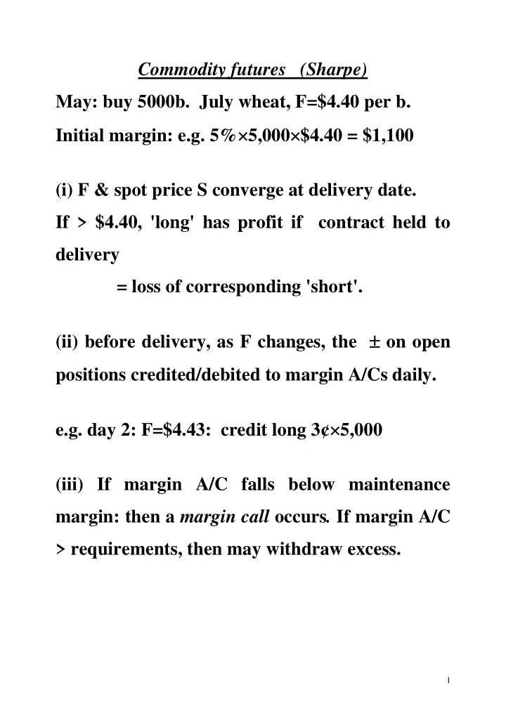
Commodity futures (Sharpe) May: buy 5000b. July wheat, F=$4.40 per b. Initial margin: e.g. 5%5,000$4.40 = $1,100 (i) F & spot price S converge at delivery date. If > $4.40, 'long' has profit if contract held to delivery = loss of corresponding 'short'. (ii) before delivery, as F changes, the  on open positions credited/debited to margin A/Cs daily. e.g. day 2: F=$4.43: credit long 3¢5,000 (iii) If margin A/C falls below maintenance margin: then a margin call occurs. If margin A/C > requirements, then may withdraw excess.

2

(iv) Suppose F = $4.50 in June. Net credit since May: 5,00010c. = $500

• Either close out, by cash settlement: i.e. sell

5,000b. July wheat, and, close margin A/C including  interest and profit of $500.

• Or withdraw all/part of $500, and continue.

(v) At delivery all open positions must be closed

• Either sell 5,000b. July wheat futures at delivery

(cash settlement)

• Or take delivery of 5,000 b. at settlement price.

3

Hedging interest rates (1) Debt to roll over in 1 period: use short hedge. Debt instrument: discount bond, which matures at par (100) in 1 period's time, when you will redeem it & sell another. Futures contracts are written on these bonds, which happen to deliver in one period from now. Initially, S=92, F=94. Sell one contract: locks in R= 6

94100% on loan starting at the delivery date.

Some possibilities: at delivery, (a) S=F=91. Close at =3. Sell bond for cash 91,

• r

(b) S=F=95. Close at =1. Sell bond for cash 95. In all cases, in effect, price of 94 locked in; alternatively, make deliverysame result.

4

Hedging A perfect hedge is unlikely

• at delivery, F=S for delivery grade;
• but (a) the position being hedged might not be

in this grade (quality; also, for commodities, location) ['Cross hedging'];

• (b) futures contracts relate to standardized

quantities;

• & (c) delivery dates of futures contracts may

differ from those of actuals activities;

• (a), (b) & (c)  'basis risk' (see later);
• 'marking to market' & initial margin  

interest.

5

Hedging interest rates (2) As (1), except delivery date assumed much later than 'roll over'. Basis FS=9492=2 initially. Sell 1 contract, & close out on rollover date. If e.g. F=97 then, then loss = 3. If basis = 2 (as initially), then S=95 at that point. Sell bond for 95, meet margincall of 3. Net receipts 92. Generally, net receipts= S1(F1F0)= F0(F1S1) Iff the basis remains constant at (F0S0) then net receipts = S0

6

Hedging to minimize risk The optimal hedge-ratio h* of futures contracts to 'actuals' exposure minimizes the variance of the change in the value V of the hedged position

• ver the life of the hedge (Hull, ch. 3.4).

V = S  hF; and var(V)= S

2 + h2F 2  2hSF, so

var h = 2hF

2  2SF

= 0 (for a min.) So h* =  S F If =1 & S=F : then h* = 1. If 1 & SF with at least one strict: h*<1:

• interpretation: hedged & unhedged positions

are different assets, and each earns its position in an optimal portfolio. var(V) h* h

7

Arbitrage (ignore 'margin' issues) A riskless discount bond: S=95, Maturity after 1 period. F=106 RF=10% p.p. Assertion: F too high, S too low.

• borrow 95 for 1 period @ RF
• buy 1 bond
• sell 1 futures contract.

After 1 period, repay 951.1 = 104.50 + deliver on the futures contract = S1 + profit on futures = (106S1) (equivalently cash-settle the futures contract at profit 106S1 and sell the bond 'cash' for S1) Profit 1.50 arises because S(1+RF) < F i.e. cost of carry RFS < FS basis To exclude arbitrage, need "=".

8

Problems with cash-and-carry arbitrage (1) Initial margin + marking to market  interest . (2) Dividends: cost of carry becomes RFS  FV(dividend). (3) Bid-ask spreads, transactions costs, taxes. (4) Arbs not the only transactors. Some deviation likely, but once basis and cost of carry get too far apart, arbitraging ('programme trading') begins, until:

• 1. Long underlying+short futures+borrow=0
• 2. Short underlying+long futures+lending=0

e.g. If index futures reach large enough discount

• v. index: sell stock, buy futures and buy T-bills.

From 1. short index futures=short stock+lending, & 2., long index futures=long stock+borrowing. Implications for portfolio rebalancing?

9

Portfolio insurance

• We know that, for some m>1,

1 stock L. + m calls S. = riskless

• Also, by put-call parity,

m stock L. + m calls S.+ m puts L. = riskless Subtracting the first from the second, L. stock +L. puts = L. riskless bond

• r L. puts = S. stock + L. bonds:

i.e. synthetic puts. Problem: short stock requirement. Solution: use short futures. We can synthesize puts on the stock index, provided cash-and-carry arbitrage is respected. See problem.

10

Futures prices and E(S) (Hull 5.14) Suppose that you speculate on a rise in the price S of an asset, taking a long futures position, while putting an amount PV(F) into the riskless asset. At delivery, cash-settle, with profit = S1F (equivalently, take delivery & sell for cash) + matured value of bond +F = S1 Initially E(PV)= F/(1+RF) + E(S1)/(1+k) where k is risk-adjusted. If E(PV)=0, then: E(S1)/(1+k)=F/(1+RF) or E(S1)=F(1+k)/(1+RF) If S1 is uncorrelated with the market, the speculation has no systematic risk, k=RF, & E(S1)=F. If S1 is positively correlated with the market, k>RF, and E(S1)>F.

11

Derivatives: extensions European options on assets paying a continuous dividend yield at the rate q (Hull, ch. 16.3) Replace S with SeqT in Black & Scholes. Logic: suppose that the underlying cash-flows grow at the cts. rate g, with/without dividends. With dividends, ST = Se(gq)T = (SeqT)egT i.e. buying dividend-paying stock for S is like buying non-dividend-paying stock for (SeqT). Applications: (Hull ch. 16, 17) Options on futures; Currency options; also: Interest-rate caps (Hull, ch. 28.2).

12

Options on futures Recall: F=S(1+RF)T or F = SeR

FT in cts. time.

In B&S, replace S with FeR

FT:

Black's model: Hull, ch. 17.8. European currency options Currency is like a stock with a known dividend yield: the foreign riskless rate. Puts & calls are options to buy/sell €1 at an exercise price $E. Other variables: $S, $F (fwd), $p, $c, R$. In B&S, replace S with SeR€T.

13

Put-call parity: Buy a call, write a put, at same E, & sell €1 fwd. Value at expiry S>E S<E Call SE Put (ES) Fwd FS FS Total FE FE Riskless return if FE>0, so arbitrage  cp = FE 1+R$ * This is put-call parity * What if FE<0? =0? what if cp  FE 1+R$? * What assumptions have I made?

14

Strategies involving currency options

• L. call+S. put+S. Fwd = riskless bond;
• S. call+L. put+L. fwd = riskless bond.

Any one instrument (S.or L.) may be synthesized from the other three. [Q. - using p.c.p. for options on stock, how could you synthesize a short-stock position?] NB: put on $ = call on €; call on $ = put on €.

15

Caps (Hull, ch. 28) I face n successive quarterly interest payments

• n a loan of size L. Rk = 3-mo Libor at stage k,

and R= min(Rk,RX) where RX is the cap rate. At t=k+1, the writer pays: 0.25L.max(RkRX,0). This is a European call option on a future (or rather forward) interest rate. Interest rate swaps (Hull, ch. 7) Borrowing rates Type A's B's Fixed X X+1.2% Floating L(ibor)+0.3% L+1%= L+0.3%+0.7% Both types cheaper for A; 0.7%<1.2% so B has a comparative advantage in floating. B wants fixed rate, A wants floating.

16

A borrows €1m at X (fixed), B borrows €1m at L+1% (floating). A pays B periodically at Libor on €1m. B pays A at Xx, where x is an agreed margin. A's net cost is L+x, a floating rate. B's net cost is X+1% x, a fixed rate. B gains if x>0. Need x<0.3% for A to gain also. Total gain: (0.3%x)+(1.2%1%+x)=1.2% 0.7% X L+1% L Xx A B