Comments on Sigma Filter Degradation of a smoothed image is due to - PowerPoint PPT Presentation

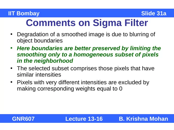
IIT Bombay Slide 31a Comments on Sigma Filter • Degradation of a smoothed image is due to blurring of object boundaries • Here boundaries are better preserved by limiting the smoothing only to a homogeneous subset of pixels in the neighborhood • The selected subset comprises those pixels that have similar intensities • Pixels with very different intensities are excluded by making corresponding weights equal to 0 GNR607 Lecture 13-16 B. Krishna Mohan

IIT Bombay Slide 32 Lee filter Simple Lee filter • g ij = f mean + k.(f ij – f mean ) • k varies between 0 and 2  k = 0, g ij = f mean  simple averaging  k = 1, g ij = f ij  no smoothing at all  k = 2, g ij = f ij + (f ij – f mean ) Interpretation of (f ij – f mean ) ??? GNR607 Lecture 13-16 B. Krishna Mohan

IIT Bombay Slide 33 Lee filter a. Original image b. Wallis filter c. K=2 d. K=3 e. K=0.5 f. K=0 GNR607 Lecture 13-16 B. Krishna Mohan

IIT Bombay Slide 34 General form of Lee filter • The general form of Lee filter is given by = + − g f k ( f f ) ij mean ij ij mean • k ij is given by σ 2 ij = k ij σ + σ 2 2 2 f mean v ij • Greater noise, smaller k ij , hence more smoothing GNR607 Lecture 13-16 B. Krishna Mohan

IIT Bombay Slide 34a Comments on General form of Lee filter • Noise variance has to be estimated from homogeneous areas • Unless noise variance is very low, this filter smoothes the image like average filter σ 2 ij = k ij σ + σ 2 2 2 f mean v ij • Greater noise, smaller k ij , hence more smoothing GNR607 Lecture 13-16 B. Krishna Mohan

IIT Bombay Slide 35 Gradient Inverse Filter • The gradient inverse filter applies weights to the neighbors in an inverse proportion to their difference to the central pixel (i,j)’s gray level • Let u(i,j,k,l)= 1 + + ≠ ( , ) | if f i , ( k j , l ) f i j ( , ) + + − | f i ( k j , l ) f i j • Else, u(i,j,k,l) = 2.0 GNR607 Lecture 13-16 B. Krishna Mohan

IIT Bombay Slide 36 Gradient Inverse Filter • The gradient inverse filter is defined by =+ =+ = ∑ ∑ k w l w g h f − − i j , i j k l , , , i k j l , =− =− k w l w • h i,j,k,l = 0.5 (weight for the centre pixel) ∑ u • h i,j,k,l = 0.5[u i,j,k,l / ] i,j,k,l k,l GNR607 Lecture 13-16 B. Krishna Mohan

IIT Bombay Slide 37 K-Nearest Neighbor algorithm • K -nearest neighbor average: compute equally weighted average of k -nearest neighbors – k neighbors whose gray levels are closest to the central pixel in the neighborhood • Sort the neighbors on the basis of similarity of gray level to the central pixel • Compute the average of K neighbors whose gray levels are closest GNR607 Lecture 13-16 B. Krishna Mohan

IIT Bombay Slide 38 Example Consider the neighborhood 33 41 37 32 46 39 30 29 28 K = 4 Closest 4 gray levels to 46 are 41, 39, 37, 33 Including the central pixel, the average is (1/5)(46 + 41 + 39 + 37 + 33) = 39.20 ~ 39 GNR607 Lecture 13-16 B. Krishna Mohan

IIT Bombay Slide 39 Non-linear filtering • Nonlinear filters have certain advantages over linear filters when dealing with noise • Common examples are the rank order filters • A typical rank order filter is of the form • g ij = H[f i,j,k,l ], where H represents a user- specified rank criterion GNR607 Lecture 13-16 B. Krishna Mohan

IIT Bombay Slide 40 Rank filtering • Modal filter • Central pixel is assigned the gray level that occurs most frequently in the neighborhood • g ij = mode {f i-k,j-l | k,l=-w, …, o, …, w} • e.g., f n = 11 12 14 15 12 16 11 15 15 • 12 is replaced by 15, which occurs most frequently in the neighborhood GNR607 Lecture 13-16 B. Krishna Mohan

IIT Bombay Slide 41 Median Filter • Median filter is the most commonly used non-linear filter for image smoothing • When the image is corrupted by random salt-and-pepper noise, median operation is very effective in removing the noise, without degrading the input image • g ij = median {f i-k,j-l | k,l=-w, …, o, …, w} GNR607 Lecture 13-16 B. Krishna Mohan

IIT Bombay Slide 42 Mean v/s Median filter • Consider an example: • 15 17 16 15 17 17 • 18 17 15 157 18 15 • 17 14 16 17 14 16 • Case 1 Case 2 • Mean=16 Mean=32 • Median=16 Median=17 • In arithmetic averaging, noise is distributed over the neighbours • In median filtering, the extreme values are pushed to one end of the sequence after sorting, hence ignored when filtered GNR607 Lecture 13-16 B. Krishna Mohan

IIT Bombay Slide 43 Algorithm • Consider the size of the window around the pixel • Collect all the pixels in the window and sort them in ascending / descending order • Select the gray level after sorting, according to the rank criterion • It can easily be verified that median and mode filters are nonlinear, according to the definition of linearity GNR607 Lecture 13-16 B. Krishna Mohan

IIT Bombay Slide 44 Median filtering Example here is over 7x7 neighborhood Example GNR607 Lecture 13-16 B. Krishna Mohan

IIT Bombay Slide 45 Trimmed Mean Filter • Trimmed-Mean Operator: • trimmed-mean: first k and last k gray levels not used • trimmed-mean: equal weighted average of central N-2k elements − 1 N k ∑ = z x trimmed mean ( n ) − N 2 k = + n 1 k GNR607 Lecture 13-16 B. Krishna Mohan

IIT Bombay Slide 46 Some Comments • Shift variant filters can adapt to the image conditions better • More computations are involved in shift variant filtering • Gaussian smoothing has some optimal properties for which it is popular • Degree of smoothing can be controlled by varying the width σ of the Gaussian filter GNR607 Lecture 13-16 B. Krishna Mohan

IIT Bombay Slide 47 Comments contd… • Simple averaging type filters fare poorly in case of signal dependent noise • Particularly with SAR images noise suppression is challenging • Noise filtering is performed in case of SAR prior to image formation or after image formation • Shift variant and nonlinear filters more successful with SAR images GNR607 Lecture 13-16 B. Krishna Mohan

IIT Bombay Slide 48 Comments contd… • An important requirement of image smoothing: the sharpness in the image should be least affected • Many comparative studies to evaluate methods • Estimating noise statistics key to improving quality of data like SAR images • Additional techniques – based on mathematical morphology GNR607 Lecture 13-16 B. Krishna Mohan

Edge Enhancement Methods

IIT Bombay Slide 49 Edge • Edge: boundary where brightness values significantly differ among neighbors edge: brightness value appears to abruptly jump up (or down) GNR607 Lecture 13-16 B. Krishna Mohan

IIT Bombay Slide 50 Original image (left), Sharpened Image (right) GNR607 Lecture 13-16 B. Krishna Mohan

IIT Bombay Slide 51 Edge Detection Essential to mark the boundaries of objects Area, shape, size, perimeter, etc. can be computed from clearly identified object boundaries Intensity / color / texture / surface orientation gradient employed to detect edges Gradient magnitude denotes the strength of edge Gradient direction relates to direction of change of intensity / color GNR607 Lecture 13-16 B. Krishna Mohan

IIT Bombay Slide 53 Different Edges A Different colors Different Intensities GNR607 Lecture 13-16 B. Krishna Mohan Different brightness