Combination of Independent Component Analysis and statistical - PowerPoint PPT Presentation
Combination of Independent Component Analysis and statistical modeling for the identification of metabonomic biomarkers Rjane Rousseau (Institut de Statistique, UCL, Belgium) Joint work with Bernadette Govaerts and Michel Verleysen (UCL)
Combination of Independent Component Analysis and statistical modeling for the identification of metabonomic biomarkers Réjane Rousseau (Institut de Statistique, UCL, Belgium) Joint work with Bernadette Govaerts and Michel Verleysen (UCL) Rousseau Réjane – 24/09/2008
Metabonomics and biomarker identification What is metabonomics ? The study of biological responses to a stressor (ex: drug, disease) in the level of metabolites Metabonomics in practice Biofluid 1 H-NMR or Mass (e.g. Urine spectroscopy New Plasma…) Whithout contact One metabolite = several peaks with specific positions in the spectrum Biomarker identification Find which metabolite or which part of the spectrum is alterated by a factor of interest (drug, disease…) Objective of the talk: to propose a methodology combining ICA and statistical modeling for biomarker identification in 1 H-NMR spectroscopy. Rousseau Réjane – 24/09/2008
Outline of the talk • � Typical steps of a metabonomic study for the identification of biomarkers • � Overview of the methodology based on ICA and statistical modeling • � Data used in the talk • � Details of the methodology Step I : Dimension reduction by ICA Step II: Mixed statistical modeling of ICA mixing weights Step III: Selection of significant sources (biomarkers) Step IV: Visualization of biomarkers and factor effects • � Conclusions. Rousseau Réjane – 24/09/2008
Typical steps of a metabonomic study Collection of biofluid samples under different conditions Factors: drug, time, ph, temperature, … 1 H-NMR Postprocessing analysis FT Spectral data PCA X ( n x m ) n samples n time signals n spectra Rousseau Réjane – 24/09/2008
Typical steps of a metabonomic study Spectral PCA: data � � Reduction of the dimension to obtain uncorrelated principal components X (nxm) � � Examination of the 2 first components to identify biomarkers Score plot Loadings L1 L2 ex: this peak plays an important role ex: colors = 4 groups of disease Identification of biomarker This is only powerful if the biological question is related to the highest variance in the dataset! Rousseau Réjane – 24/09/2008
Methodology based on ICA and statistical modeling Step I : Dimension reduction by ICA X TC = S . A T Components Weights � quantity Examination of the ALL components: to visualize unconnected molecules in samples Step II: Mixed statistical modeling + � A T = Z 1 � + Z 2 � + on ICA mixing weights Step III: Selection of sources S* � S identification of biomarkers Step IV: Visualization of the effect of the factor of interest on the biomarkers Rousseau Réjane – 24/09/2008
Data used in this talk Hippurate • � Prepared samples Age � � to know the spectral regions that should be identified as biomarkers � � Mixtures of urine with citrate and hippurate � � 14 experimental conditions – 2 replicates per condition = 28 samples Citrate • � Spectra postprocessing Drug dose � � Using Bubble a tool developped by Eli Lilly optimised for urine samples � � Normalisation : unit sum - Resolution : 600ppms • � Typical spectrum = Natural urine + Hippurate + Citrate Hypothetical question � � Assimilate the concentration of citrate as a drug dose received by the subject of hippurate as the age of the subject � � Goal = to find a biomarker for the drug dose i.e. discover « automatically » the citrate peak from the 28 spectra. Rousseau Réjane – 24/09/2008
Methodology based on ICA and statistical modeling Step I : Dimension reduction by ICA X TC = S.A T � � What is ICA? � � Dimension reduction by ICA � � Illustration on the example � � Comparison of ICA and PCA Step II: Mixed statistical modeling of ICA mixing weights Step III: Selection of significant sources (biomarkers) Step IV: Visualization of biomarkers and factor effects Rousseau Réjane – 24/09/2008
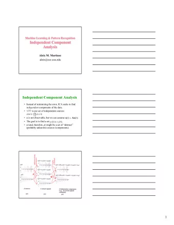
Step I : What is Independent component analysis (ICA)? � � The idea: • � Each observed vector of data (spectrum) is a linear combination of unknown independent (not only linearly independent) components • � The ICA provides the independent components (sources, s k ) which have created a vector of data and the corresponding mixing weights a ki . � � How do we estimate the sources? with linear transformations of observed signals that maximize the independence of the sources. � � How do we evaluate this property of independence? Using the Central Limit Theorem (*), the independence of sources components can be reflect by non-gaussianity. Solving the ICA problem consists of finding a demixing matrix which maximises the non- gaussianity of the estimated sources under the constraint that their variances are constant. � � Fast-ICA algorithm: - uses an objective function related to negentropy - uses fixed-point iteration scheme . * almost any measured quantity which depends on several underlying independent factors has a Gaussian PDF Rousseau Réjane – 24/09/2008
Step I : dimension reduction by ICA : X (nxm) n spectra defined by m variables ex: (28x600 ) Transposition X T (mxn) Centering By spectrum !! X TC = S.A T + E X TC (mxn) “Whitening”: Each spectrum is a weighted sum of the Goals independent spectral expressions • � work on an orthogonal matrix which each one can correspond to • � Reduce the number of source to calculate an independent (composite) T (mxq) = X TC . P metabolite contained in ICA the studied sample. (a T , weight � quantity) S (mxq) = X TC . P.W = X TC . A Rousseau Réjane – 24/09/2008
Step I : Example X TC (600 x 28) = S (600 x 6) A T (6x28) x TC 1 x TC s 1 s 2 s 3 s 4 s 5 s 6 28 s 1,1 a t at 1,1 ..... s 1,6 at 1,28 1 ... a t 2 .... a t s ij = 3 .... a t 4 a t 5 a t 6 at 6,1 s 600,1 Urine + citrate + hippurate Rousseau Réjane – 24/09/2008
Mixing weigthsA T Sources : S (600 x 6) 28 spectra Natural urine a T 2,8 Citrate Hippurate Rousseau Réjane – 24/09/2008
Step I: Comparison with the usual PCA Similarities : projection methods linearly decomposing multi-dimensional data into components . • � Differences: • � � � ICA uses X T (mxn) ( PCA uses X (nxm) ) � � The number of sources, q , has to be fixed in ICA � � Sources are not naturally sorted according to their importance in ICA � � The independence condition = the biggest advantage of the ICA: - independent components (ICA) are more meaningful than uncorrelated components (PCA) - more suitable for our question in which the component of interest are not always in the direction with the maximum variance. PCA ICA 1 2 Natural urine Rousseau Réjane – 24/09/2008
PCA ICA Hippurate & Citrate Natural urine Loading 1 s 1 Citrate Loading 2 s 2 Hippurate & Citrate Hippurate Loading 3 s 3 PC2 a T 3 PC1 a T 2 Rousseau Réjane – 24/09/2008
Methodology based on ICA and statistical modeling Step I : Dimension reduction by ICA X TC (600x28) = S . A T Some of these sources present the biomarkers. Which ones? Step II: Mixed statistical modeling on ICA mixing weights + � A T = Z 1 � + Z 2 � + Step III: Selection of significant sources (biomarkers) S* � S Step IV: Visualization of biomarkers and factor effects Rousseau Réjane – 24/09/2008
Step II: statistical modeling of ICA mixing weights � � For each of the q sources s j , we assume a linear relation between its vector of weights and the design variables: a j = Z 1 � j + Z 2 � j + � j Mixing weights matrix for matrix for for source j the covariates the covariates with fixed effects with random effects � � Models with fixed and random effects covariates : Mixed model: a j = Z 1 � j+ Z 2 � j + � j � � Models with only random effects covariates : a j = Z 2 � j + � j � ex: biomarker to explore variance component (machines, subjects, laboratories) � � Models with only fixed effects covariates : a j = Z 1 � j + � j • � Case 1: categorical covariates: ANOVA � ex: biomarker to discriminate 3 groups of subjects: disease1, disease2 & sane • � Case 2: quantitative covariates : linear regression � ex: biomarker to explore the severity of an illness, the concentration of a drug Rousseau Réjane – 24/09/2008
Step II: Fit a model: example • � For each of the q = 6 recovered s j, we construct a multiple linear regression model with 2 fixed quantitative covariates and no interaction: a j = � j0 + � j1 y 1 + � j2 y 2 + � j Mixing weights Drug dose Age for source j (covariate of interest) For each of the 6 sources s j , the fitted model by least square technique is : • � â j = b j0 + b j1 y 1 + b j2 y 2 s 2 : Citrate Ex: a 2 Drug dose Age (y 2 ) (y 1 ) Rousseau Réjane – 24/09/2008
Methodology based on ICA and statistical modeling Step I : Dimension reduction by ICA Step II: Mixed statistical modeling on ICA mixing weights X TC (600x28) = S . A T b 11 M b 21 O D b 31 E b 41 L b 51 S b 61 Step III: Selection of significant sources (biomarkers) S* � S Step IV: Visualization of biomarkers and factor effects Rousseau Réjane – 24/09/2008
Recommend
More recommend
Explore More Topics
Stay informed with curated content and fresh updates.
