Coarsening of three-dimensional structured and unstructured grids - PowerPoint PPT Presentation
Coarsening of three-dimensional structured and unstructured grids for subsurface flow Jrg Espen Aarnes and Vera Louise Hauge SINTEF ICT, Norway Yalchin Efendiev Texas A&M University, Texas, USA Task: Given ability to model velocity on
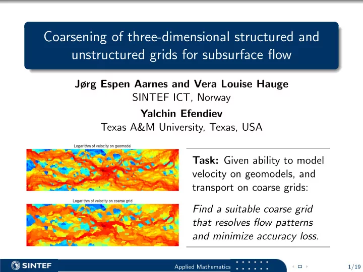
Coarsening of three-dimensional structured and unstructured grids for subsurface flow Jørg Espen Aarnes and Vera Louise Hauge SINTEF ICT, Norway Yalchin Efendiev Texas A&M University, Texas, USA Task: Given ability to model velocity on geomodels, and transport on coarse grids: Find a suitable coarse grid that resolves flow patterns and minimize accuracy loss . Applied Mathematics 1/19
Motivation Today: Geomodels too large and complex for flow simulation: Upscaling performed to obtain Simulation grid(s). Effective parameters and pseudofunctions. Reservoir simulation workflow − → − → − → Upscaling Geomodel Flow simulation Management Tomorrow: Earth Model shared between geologists and reservoir engineers — Simulators take Earth Model as input, users specify grid-resolution to fit available computer resources and project requirements. Applied Mathematics 2/19
Objectives Main objective: Develop a generic grid coarsening algorithm for reservoir simulation that resolves dominating flow patterns. – generic: one implementation applicable to all types of grids. – resolve flow patterns: separate high flow and low flow regions. Secondary objective: Reduce the need for pseudofunctions. Applied Mathematics 3/19
Simulation model and solution strategy Simulation model Pressure equation and component mass-balance equations Darcy velocity v , Primary variables: Liquid pressure p o , Saturations s j , j =aqueous, liquid, vapor. Iterative sequential solution strategy: v ν +1 = v ( s j,ν ) , s j,ν +1 = s j ( p o,ν +1 , v ν +1 ) . p o,ν +1 = p o ( s j,ν ) , (Fully implicit with fixed point rather than Newton iteration). Applied Mathematics 4/19
Simulation model and solution strategy Simulation model Pressure equation and component mass-balance equations Darcy velocity v , Primary variables: Liquid pressure p o , Saturations s j , j =aqueous, liquid, vapor. Iterative sequential solution strategy: v ν +1 = v ( s j,ν ) , s j,ν +1 = s j ( p o,ν +1 , v ν +1 ) . p o,ν +1 = p o ( s j,ν ) , (Fully implicit with fixed point rather than Newton iteration). Advantages with sequential solution strategy: Grid for pressure and mass balance equations may be different. Multiscale methods may be used to solve pressure equation. Pressure eq. allows larger time-steps than mass balance eqs. Applied Mathematics 4/19
Discretization Pressure equation: Solution grid: Geomodel — no effective parameters. Discretization: Multiscale mixed / mimetic method Coarse grid: obtained by up-gridding in index space Mass balance equations: Solution grid: Non-uniform coarse grid. Discretization: Two-scale upstream weighted FV method — integrals evaluated on geomodel. Pseudofunctions: No. Applied Mathematics 5/19
Generation of coarse grid for mass balance equations Coarsening algorithm 1 Separate regions with different magnitude of flow. 2 Combine small blocks with a neighboring block. 3 Refine blocks with too much flow. 4 Repeat step 2. Example: Layer 1 SPE10 (Christie and Blunt), 5 spot well pattern. Applied Mathematics 6/19
Grid generation procedure Example: Layer 1 SPE10 (Christie and Blunt), 5 spot well pattern Separate: Define g = ln | v | and D = (max( g ) − min( g )) / 10. Region i = { c : min( g ) + ( i − 1) D < g ( c ) < min( g ) + iD } . Initial grid: connected subregions — 733 blocks Applied Mathematics 7/19
Grid generation procedure Example: Layer 1 SPE10 (Christie and Blunt), 5 spot well pattern Separate: Define g = ln | v | and D = (max( g ) − min( g )) / 10. Region i = { c : min( g ) + ( i − 1) D < g ( c ) < min( g ) + iD } . Initial grid: connected subregions — 733 blocks Merge: If | B | < c , merge B with a neighboring block B ′ with 1 1 � � ln | v | dx ≈ B ′ ln | v | dx | B ′ | | B | B Step 2: 203 blocks Applied Mathematics 7/19
Grid generation procedure Example: Layer 1 SPE10 (Christie and Blunt), 5 spot well pattern Refine: If criteria — � B ln | v | dx < C — is violated, do Start at ∂B and build new blocks B ′ that meet criteria. Define B = B \ B ′ and progress inwards until B meets criteria. Step3: 914 blocks Applied Mathematics 8/19
Grid generation procedure Example: Layer 1 SPE10 (Christie and Blunt), 5 spot well pattern Refine: If criteria — � B ln | v | dx < C — is violated, do Start at ∂B and build new blocks B ′ that meet criteria. Define B = B \ B ′ and progress inwards until B meets criteria. Step3: 914 blocks Cleanup: Merge small blocks with adjacent block. Final grid: 690 blocks Applied Mathematics 8/19
Example: Log of velocity magnitude on different grids Applied Mathematics 9/19
Layer 68 SPE10, 5 spot well pattern Geomodel: 13200 cells Coarse grid: 660 cells Coarse grid: 649 cells Coarse grid: 264 cells Coarse grid: 257 cells Applied Mathematics 10/19
Numerical examples Performance studies Experimental setup: Model: Incompressible two-phase flow (oil and water). Initial state: Completely oil-saturated. Relative permeability: k rj = s 2 j , 0 ≤ s j ≤ 1. Viscosity ratio: µ o /µ w = 10. Error measures: (Time measured in PVI) � 1 � S ( · ,t ) − S ref ( · ,t ) � L 1(Ω) Saturation error: e ( S ) = dt. 0 � S ref ( · ,t ) � L 1(Ω) e ( w ) = � w − w ref � L 2 ([0 , 1]) / � w ref � L 2 ([0 , 1]) . Water-cut error: Applied Mathematics 11/19
Example 1: Geomodel = individual layers from SPE10 5-spot well pattern, upscaling factor ∼ 20 Saturation error for each of the 85 layers in the SPE10 model 0.5 Non−uniform coarsening Geomodel: Uniform coarsening 0.4 60 × 220 × 1 0.3 e(S) 0.2 0.1 Uniform grid: 0 0 10 20 30 40 50 60 70 80 Layer 15 × 44 × 1 Water−cut error for each of the 85 layers in the SPE10 model 0.2 Non−uniform coarsening Uniform coarsening 0.15 e(w) Non-uni. grid: 0.1 0.05 619–734 blocks 0 0 10 20 30 40 50 60 70 80 Layer Observations: First 35 layers smooth ⇒ Uniform grid adequate. Last 50 layers fluvial ⇒ Uniform grid inadequate. Non-uniform grid gives consistent results for all layers. Applied Mathematics 12/19
Example 2: Geomodel = stack of five layers from SPE10 5-spot well pattern, upscaling factor ∼ 100 Saturation error for each of the 17 stacks of five consecutive layers in the SPE10 model 0.8 Non−uniform coarsening Uniform coarsening 0.7 Geomodel: 0.6 0.5 e(S) 60 × 220 × 5 0.4 0.3 0.2 0.1 Uniform grid: 0 2 4 6 8 10 12 14 16 18 Stack 15 × 44 × 1 Water−cut error for each of the 17 stacks of five consecutive layers in the SPE10 model Non−uniform coarsening Uniform coarsening 0.25 0.2 Non-uniform grid: e(w) 0.15 0.1 655–714 blocks 0.05 0 0 2 4 6 8 10 12 14 16 18 Stack Observations: Uniform grid inadequate, also for stacks from layers 1–35 — lognormal mean of permeability in layers varies significantly. Non-uniform grid gives consistent results for all stacks. Applied Mathematics 13/19
Example 3: Geomodel = unstructured corner-point grid 20 realizations from lognormal distribution, Q-of-5-spot well pattern, upsc. factor ∼ 25 ⇐ 2 realizations. Geomodel: 15206 cells Saturation error for 20 stochastic permeability realizations Water−cut error for 20 stochastic permeability realizations 0.7 0.3 Non−uniform coarsening Non−uniform coarsening Uniform grid: Uniform coarsening Uniform coarsening 0.6 0.25 Average saturation error for µ o =10 µ w Water−cut error for µ o =10 µ w 838 blocks 0.5 0.2 0.4 0.15 0.3 0.1 Non-uni. grid: 0.2 0.05 647–704 blocks 0.1 0 0 2 4 6 8 10 12 14 16 18 20 0 2 4 6 8 10 12 14 16 18 20 Observations: Coarsening algorithm applicable to unstructured grids — accuracy consistent with observations for SPE10 models. Results obtained with uniform grid (in index space) inaccurate. Applied Mathematics 14/19
Example 4: Geomodel = four bottom layers from SPE10 Robustness with respect to degree of coarsening, 5-spot well pattern Number of cells in grid (upscaling factor 4–400) Uniform grid 30x110x4 20x55x4 15x44x2 10x22x2 6x22x1 13200 4400 1320 440 132 Non-U. grid 7516 3251 1333 419 150 Average saturation error Water−cut error 0.5 0.25 Non−uniform coarsening Non−uniform coarsening 0.45 Uniform coarsening Uniform coarsening 0.4 0.2 0.35 0.3 0.15 0.25 0.2 0.1 0.15 0.1 0.05 0.05 0 0 30x110x4 20x55x4 15x44x2 10x22x2 6x22x1 30x110x4 20x55x4 15x44x2 10x22x2 6x22x1 Observations: Non-uniform grid gives better accuracy than uniform grid. Water-cut error almost grid-independent for non-uniform grid. Applied Mathematics 15/19
Example 5: Geomodel = four bottom layers from SPE10 Robustness with respect to well configuration, upscaling factor ∼ 40 A B C D E = Injector = Producer Wellpatterns Average saturation error Water−cut error 0.5 0.15 Uniform grid: Non−uniform coarsening Non−uniform coarsening Uniform coarsening Uniform coarsening 0.45 0.4 15 × 44 × 2 0.35 0.1 0.3 0.25 0.2 Non-uniform grid 0.05 0.15 0.1 ∼ 1320 blocks 0.05 0 0 A (1333) B (1355) C (1348) D (1347) E (1337) A (1333) B (1355) C (1348) D (1347) E (1337) Non-uniform grid gives better accuracy than uniform grid — substantial difference in water-cut error for all cases. Applied Mathematics 16/19
Recommend
More recommend
Explore More Topics
Stay informed with curated content and fresh updates.
