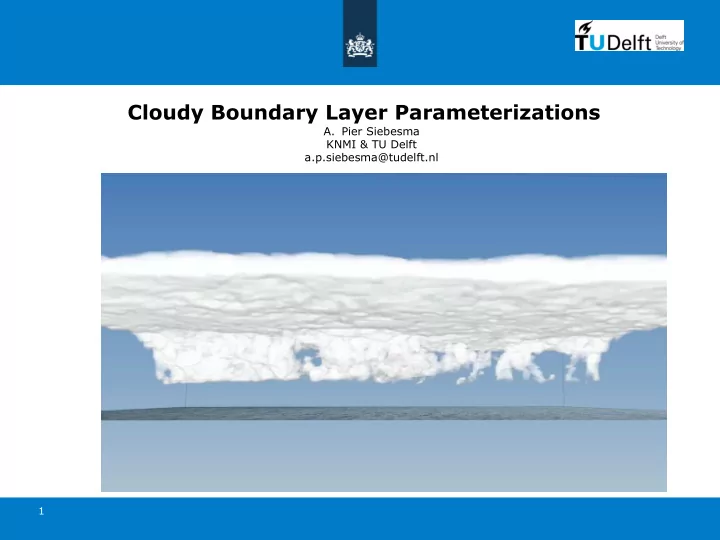
Cloudy Boundary Layer Parameterizations A. Pier Siebesma KNMI & - PowerPoint PPT Presentation

Cloudy Boundary Layer Parameterizations A. Pier Siebesma KNMI & TU Delft a.p.siebesma@tudelft.nl 1

The role of the cloudy boundary layer (1) Transport of heat moisture, momentum Bony et al., Nature GeoSciences, 2015 Vertical transport of heat, moisture and momentum

The role of the cloudy boundary layer (1) Interaction with radiation (dominated by SW cooling) Wild et al. Climate Dyn. (2013) Reflecting, absorbing lw radiation, emitting lw radiation.

�������� � ��������� � � ���� � ���� � � � � �� ���������� �������� ��� ��������� � ������ � � � ������� Large(st) source of uncertainty in Climate Models Uncertainty in Equilibrium Climate Sensitivity (ECS) can be largely attributed to uncertainty in low cloud feedback a b Amplifying Damping Higher ECS Lower ECS feedback feedback 5 600 2060 Allowable CO 2 concentration (ppm) 4 2 1 29 5 28 Year of crossing 2 °C threshold ks 27 26 25 24 22 ly, 4 21 20 3 550 2051 ECS (K) 19 18 18 16 11 9 8 14 6 15 14 17 16 13 10 13 12 7 3 22 12 11 9 10 20 6 78 15 500 2042 26 25 23 24 5 27 19 4 28 21 3 29 2 1 2 1/5 1/4 1/3 1/2 –1 –0.5 0 0.5 g 1/ECS (K –1 ) Low-cloud reflectance change (% K –1 ) Schneider et al. Nature Climate Change (2017)

Traditional Parameterization break-up in GCMs turbulence Resolved convection Scales clouds radiation ~ 100 km Small scales Large scales

Turbulence Parameterization (early days) Traditionally restricted to the “dry” (i.e. cloudfree ) boundary layer Rotterdam, The Netherlands

Turbulence Parameterization (evolving) Including Stratocumulus(Scu) topped BL

Turbulence Parameterization (further evolving) Including Boundary Layer (shallow) cumulus clouds

Different Parameterization Schemes have overlapping tasks (1) D t s = − ∂ p ω 0 s 0 + L ( c − e ) + Q r D t q v = − ∂ p ω 0 q 0 v − ( c − e ) D t q c = − ∂ p ω 0 q 0 c + ( c − e ) − G BL scheme X X X cloud scheme Cloud BL scheme scheme Conv scheme Conv scheme Radiation scheme Radia1on scheme

Different Parameterization Schemes sharing tasks (1) D t s = − ∂ p ω 0 s 0 + L ( c − e ) + Q r D t q v = − ∂ p ω 0 q 0 v − ( c − e ) D t q c = − ∂ p ω 0 q 0 c + ( c − e ) − G BL scheme X X X cloud scheme Cloud x x BL scheme scheme Conv scheme Conv x x x scheme Radiation scheme Radia1on x scheme

Temperature tendencies of EC-Earth (1986-2006) Atmosphere only with prescribed SST’s CONV RAD CLD BL

1. Traditional (Mixed) Boundary Layer Scheme developments parameterizations 12

Historically: The dry (convective) boundary layer Rotterdam, The Netherlands

Traditional Approach: ED Eddy-Diffusivity (1) ∂ φ w ' φ ' K ≈ − φ = { s d , q v } After: Before: z ∂ Local transport by small-scale motions, Diffusive from high values of φ towards low transport values ED: “the great equalizer”, flattening vertical profiles θ θ To be parameterized: K

Format for parameterizing eddy-diffusivity K ∂ φ w K K c w l with ʹ ʹ φ = − ≈ t z φ ∂ l(z) : typical eddy size at height z w(z) : typical vertical velocity at height z θ ρ q v θ ρ ,p

Format for length scale formulation Length scale l(z): ∂ φ w K K c w l with • Not well defined but loosely interpreted as the size of ʹ ʹ φ = − ≈ t z φ ∂ the dominant turbulent eddy at height z • Many different formulations have been proposed l(z) : typical eddy size at height z • Should match surface layer similarity w(z) : typical vertical velocity at height z θ ρ q v z θ ρ ,p l 1 = 1  z + 1 For instance: ` t �

Format for velocity scale ∂ φ w K K c w l with ʹ ʹ φ = − ≈ t z φ ∂ 1 ( ) w e u u ' ' v v ' ' w w ' ' = = + + Turbulent Kinetic Energy (TKE) : t 2 2 ⎛ ⎞ e 3/2 ∂ e ∂ u g ∂ e ∂ θ v ∂ t = K m − K h ∂ z + 2 K m ∂ z − c d ⎜ ⎟ Solved Prognostically : ℓ ∂ z θ o ⎝ ⎠ S B T D Shear Buoyancy Dissipation Transport Production Production S + B – D = 0 Or diagnostically : Or by a simple profile

2. Extension to Scu topped BL parameterizations 18

Characteristics of stratocumulus q θ v v Courtesy: B. Stevens Well mixed but only in terms of moist conserved variables : q t , θ l Turbulence also driven due to the radiative cooling L q q q = + q θ = θ − t v l l l c π p

Dry Formulation Moist Formulation 1. Allow the “test parcel” to condensate so that it can find the Scu cloud top. (at least a moist adiabat). A “dry” K-profile will detect Cloud base as inversion 2. Construct a K-profile from the surface and will only mix in the to the Scu cloud top subcloud layer 3. Apply the Eddy Diffusivity on the moist conserved variables q t and θ l 4. Translate the new values of qt and θ l back into qv and ql and Τ

Moist TKE 2 ⎛ ⎞ e 3/2 ∂ e ∂ u g ∂ e ∂ θ v • TKE equation ∂ t = K m − K h ∂ z + 2 K m ∂ z − c d ⎜ ⎟ ℓ ∂ z θ o ⎝ ⎠ 1 1 1 • length scale (moist adiabatic testparce)) = + ℓ ℓ ℓ u d • buoyancy flux: � � � w 0 θ 0 � � � = a c cld + (1 − a c ) w 0 θ 0 w 0 θ 0 clr . v v Remark 2: If vertical resolution is high enough Remark 1: Note that the cloud fraction (100m) and the scheme is well callibrated no has now entered the equations prescribed top-entrainment is necessary 800 height (m) 400 0 0 2x10 -5 -0.1 0 -0.03 0 0.03 w'q t ' (kg kg -1 )(ms -1 ) w' θ l ' (mKs -1 ) w' θ ρ ' (mKs -1 )

IFS “Dry” Formulation cloud fraction model obs model - obs Courtesy M. Kohler

“Moist” Formulation IFS cloud fraction model obs model - obs

Summary (so far) • Virtually all NWP and Climate models use an eddy-diffusivity approach to parameterize turbulent transport in the boundary layer. ∂ φ w K K c w l ʹ ʹ with φ = − ≈ t z φ ∂ • Two popular flavours: • K-profile (with aditional Ri-formulations for stable cases) (EC-Earth,IFS, Hadgem) • Simple and hence more robust formulation • Needs explicity “switching”between regimes (convective ó neutral, stable). • Needs explicit treatment of top-entrainment. • TKE schemes: (ECHAM, ARPEGE) • physically well founded • works for different stability regimes (convective, stable, neutral) • many uncertain free parameters (length scale, closures in TKE etc) • needs careful tuning for matching surface layer, top-entrainment etc …

3. Transitions to Cumulus Topped BL parameterizations 25

Transitions to cumulus topped BL. Cloud top height cumulus topped clear convec.ve Clear => Cu topped boundary layer boundary layer height Inversion Li8ing condensa.on height level (LCL) 0.5 ~ 1 km top-entrainment Scu =>Cu topped

Transitions to cumulus topped BL. Cloud top height cumulus topped clear convec.ve Clear => Cu topped boundary layer boundary layer height Inversion Li8ing condensa.on height level (LCL) 0.5 ~ 1 km top-entrainment Charactererized by “non-local” transport the case of the CBL. 1, Transport against the gradient

Leading to non-Gaussian bi-modal pdf(w,q t , θ l ) … . Cloud top height ped ayer Li8ing condensa.on level (LCL) 0.5 ~ 1 km

… . has been the main justification for mass-flux parameterizations for deep convection ( Betts 1973, Arakawa& Schubert 1974, Tiedtke 1988) e c M ( ) w ( 1 ) w w w ( ) ≈ φ − φ ʹ ʹ ʹ ʹ ʹ ʹ φ = − σ φ + σ φ + σ φ − φ c e c c e w c a a a

… and motivation of the Eddy Diffusivity – Mass Flux (EDMF) approach N ∂ φ w ' ' K M ( ) ∑ φ = − + φ − φ i i PBL z ∂ i 1 = Moist updraft Updrafts initiated from near • the surface Take care of non-local • transport in dry BL And transform into cumulus • Dry updraft if the LCL can be reached No need for trigger function • for convection K diffusion Flexible moist area fraction Top 10 % of updrafts that is explicitly modelled More on this on Wednesday Siebesma et al 2007, Neggers et al 2009

The “minimum” updraft model ( ) M ∂ φ ∂ φ − φ { } l q , Prognostic equation: c F φ = θ with ≈ − + t t z ∂ ∂ M ∂ Continuity equation: E D = − ∂ φ z ( ) ∂ c = − ε φ − φ c z ∂ M ∂ φ c E D Steady state cloud eq,: = − φ + φ ln M c ∂ z ∂ = ε − δ z ∂ Excercise!! Introduce fractional rates: ε : fractional entrainment : ε =E/M δ : fractional detrainment: δ =D/M