Classification Department Biosysteme Karsten Borgwardt Data Mining - PowerPoint PPT Presentation
Classification Department Biosysteme Karsten Borgwardt Data Mining Course Basel Fall Semester 2016 66 / 164 What is Classification? Problem Given an object, which class of objects does it belong to? Given object x , predict its class label y
Classification Department Biosysteme Karsten Borgwardt Data Mining Course Basel Fall Semester 2016 66 / 164
What is Classification? Problem Given an object, which class of objects does it belong to? Given object x , predict its class label y . Examples Computer vision: Is this object a chair? Credit cards: Is this customer to be trusted? Marketing: Will this customer buy/like our product? Function prediction: Is this protein an enzyme? Gene finding: Does this sequence contain a splice site? Personalized medicine: Will this patient respond to drug treatment? Department Biosysteme Karsten Borgwardt Data Mining Course Basel Fall Semester 2016 67 / 164
What is Classification? Setting Classification is usually performed in a supervised setting: We are given a training dataset . A training dataset is a dataset of pairs { ( x i , y i ) } n i =1 , that is objects and their known class labels. The test set is a dataset of test points { x ′ i } d i =1 with unknown class label. The task is to predict the class label y ′ i of x ′ i via a function f . Role of y if y ∈ { 0 , 1 } : then we are dealing with a binary classification problem if y ∈ { 1 , . . . , n } , (3 ≤ n ∈ N ): a multiclass classification problem if y ∈ R : a regression problem Department Biosysteme Karsten Borgwardt Data Mining Course Basel Fall Semester 2016 68 / 164
Evaluating Classifiers The Contingency Table In a binary classification problem, one can represent the accuracy of the predictions in a contingency table: y = 1 y = − 1 f ( x ) = 1 TP FP f ( x ) = − 1 FN TN Here, T refers to True , F to False , P to Positive (prediction) and N to Negative (prediction). Department Biosysteme Karsten Borgwardt Data Mining Course Basel Fall Semester 2016 69 / 164
Evaluating Classifiers Accuracy The accuracy of a classifier is defined as TP + TN TP + TN + FP + FN Accuracy measures which percentage of the predictions is correct. It is the most common criterion for reporting the performance of a classifier. Still, it has a fundamental shortcoming: If the classes are unbalanced, the accuracy on the entire dataset may look high, while being low on the smaller class. Department Biosysteme Karsten Borgwardt Data Mining Course Basel Fall Semester 2016 70 / 164
Evaluating Classifiers Precision-Recall If the positive class is much smaller than the negative class, one should rather use precision and recall to evaluate the classifier. The precision of a classifier is defined as TP TP + FP . The recall of a classifier is defined as TP TP + FN . Department Biosysteme Karsten Borgwardt Data Mining Course Basel Fall Semester 2016 71 / 164
Evaluating Classifiers Trade-off between Precision and Recall There is a trade-off between precision and recall: By predicting all points to be positive ( f ( x = 1)) one can guarantee that the recall is 1. However, the precision will then be bad. By only predicting points to be members of the positive class for which one is highly confident about the prediction, one will increase precision, but lower recall. One workaround is to report the precision recall break-even point, that is the value at which precision and recall are identical. Department Biosysteme Karsten Borgwardt Data Mining Course Basel Fall Semester 2016 72 / 164
Evaluating Classifiers Dependence on Classification Threshold TP , TN , FP , FN depend on f ( x ) where x ∈ D . The most common definition of f ( x ) is � 1 if s ( x ) ≥ θ, f ( x ) = − 1 if s ( x ) < θ, where s : D → R is a scoring function, and θ ∈ R is a threshold. As the predictions based on f vary with θ , so do TP , TN , FP , FN , and all evaluations criteria based on them. It is therefore important to report results as a function of θ whenever possible, not just for one fixed choice of θ . Department Biosysteme Karsten Borgwardt Data Mining Course Basel Fall Semester 2016 73 / 164
Evaluating Classifiers How to report results as a function of θ The efficient strategy to compute all solutions as a function of θ is to rank all points x by their score s ( x ). This ranking is a vector of length t . This ranking is a vector r of length t , whose i th element is r ( i ). We then perform the following steps: For i = 1 to t − 1 Define the positive predictions P to be the set { r (1) , . . . , r ( i ) } . Define the negative predictions N to be the set { r ( i + 1) , . . . , r ( t ) } . Compute the evaluation criteria e ( i ) of interest for P and N . Return vector e The common strategy is to compute two evaluation criteria e 1 and e 2 and to then visualize the result in a 2-D plot. Department Biosysteme Karsten Borgwardt Data Mining Course Basel Fall Semester 2016 74 / 164
Evaluating Classifiers ROC curves One popular such 2D-plot is the Receiver Operating Characteristics Curve, which represents the true positive rate versus the false positive rate . The true positive rate (or sensitivity ) is identical to the recall: TP TP + FN . That is, the fraction of positive points that were correctly classified. The false positive rate (or 1 − specificity ) is FP FP + TN That is, the fraction of negative points that were misclassified. Department Biosysteme Karsten Borgwardt Data Mining Course Basel Fall Semester 2016 75 / 164
Evaluating Classifiers ROC curves Each ROC curves starts at (0,0). If no point is predicted to be positive, then there are no True Positives and False Positives. Each ROC curve ends at (1,1). If all points are predicted to be positive, then there are no True Negatives and False Negatives. Department Biosysteme Karsten Borgwardt Data Mining Course Basel Fall Semester 2016 76 / 164
Evaluating Classifiers ROC curves The ROC curve of a perfect classifier runs through the point (0,1) - it correctly classifies all negative points (FP=0) and correctly classifies all positive points (FN=0). While the ROC curve does not depend on an arbitrarily chosen threshold θ , it seems difficult to summarize the performance of a classifier in terms of a ROC curve. Department Biosysteme Karsten Borgwardt Data Mining Course Basel Fall Semester 2016 77 / 164
Evaluating Classifiers ROC curves The solution to this problem is the Area under the Receiver Operating Characteristics (AUC), a number between 0 and 1. The AUC can be interpreted as follows: When we present one negative and one positive test point to the classifier, then the AUC is the probability with which the classifier will assign a larger score to the positive than to the negative point. The larger AUC, the better the classifier. The AUC of a perfect classifier can be shown to be 1. The AUC of a random classifier (guessing the prediction) is 0.5. The AUC of a ‘stupid’ classifier (misclassifying all points) is 0. Department Biosysteme Karsten Borgwardt Data Mining Course Basel Fall Semester 2016 78 / 164
Evaluating Classifiers Summarizing PR values 2-D plot of (recall,precision) values for different values of θ Starts at (0,1). Full precision, no recall. The precision recall break-even point is the point at which the precision-recall-curve intersects the bisecting line. The area under the precision-recall-curve (AUPRC) is another statistic to quantify the performance of a classifier. It is 1 for a perfect classifier, that is, it reaches 100% precision and 100% recall at the same time. Department Biosysteme Karsten Borgwardt Data Mining Course Basel Fall Semester 2016 79 / 164
Evaluating Classifiers Example: The Good and the Bad We are given 102 test points, 2 are positive, 100 negative. Our prediction ranks ten negative points first, then the 2 positive points, then the remaining 90 points. 1.0 1.0 0.8 0.8 True Positive Rate 0.6 0.6 Precision 0.4 0.4 0.2 0.2 0.0 0.0 0.0 0.2 0.4 0.6 0.8 1.0 0.0 0.2 0.4 0.6 0.8 1.0 Recall False Positive Rate Department Biosysteme Karsten Borgwardt Data Mining Course Basel Fall Semester 2016 80 / 164
Evaluating Classifiers What to do if we only have one dataset for training and test? If only one dataset is available for training and testing, it is essential not to train and test on the same instance, but rather to split the available data into training and test data . Splitting the dataset into k subsets and using one of them for testing and the rest for training is referred to as k-fold cross-validation . If k = n , cross-validation is referred to as leave-one-out-validation . Randomly sampling subsets of the data for training and testing and averaging over the results is called bootstrapping . Department Biosysteme Karsten Borgwardt Data Mining Course Basel Fall Semester 2016 81 / 164
Evaluating Classifiers Illustration of cross-validation: 10-fold cross-validation 1 2 3 4 5 6 7 8 9 10 1 2 3 4 5 6 7 8 9 10 Step 1 1 2 3 4 5 6 7 8 9 10 Step 2 ... ... 1 2 3 4 5 6 7 8 9 10 Step 10 Department Biosysteme Karsten Borgwardt Data Mining Course Basel Fall Semester 2016 82 / 164
Evaluating Classifiers How to optimize the parameters of a classifier? Most classifiers use parameters c that have to be set (more on these later). It is wrong to optimize these parameters by trying out different values and picking those that perform best on the test set. These parameters are overfit on this particular test dataset, and may not generalize to other datasets. Instead, one needs an internal cross-validation on the training data to optimize c . Department Biosysteme Karsten Borgwardt Data Mining Course Basel Fall Semester 2016 83 / 164
Recommend
More recommend
Explore More Topics
Stay informed with curated content and fresh updates.

![Classification Image Classification Set of predefined categories [eg: table, apple, dog, giraffe]](https://c.sambuz.com/743996/classification-s.webp)
