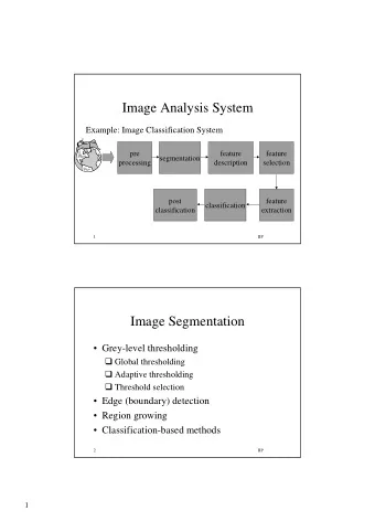
Classification of Raster Maps for Automatic Feature Extraction - PowerPoint PPT Presentation

Classification of Raster Maps for Automatic Feature Extraction Yao-Yi Chiang and Craig A. Knoblock University of Southern California 1

Motivation  Raster map is a bitmap image of a map  Raster maps are easily accessible  Contain information that is difficult to find elsewhere  Contain historical data USGS topographic map of St. Louis, MO Travel map of Tehran, Iran 2

Exploit the geospatial information in raster maps  Extracting geographic features from raster maps  Road Extraction  Text Extraction and Recognition  Building Extraction  … Text Original map Roads 3

Pre-Processing for feature extraction  Much of the feature extraction work relies on user input to extract the foreground pixels from the maps as a preprocessing step  Pre-Processing examples:  Convert to grayscale Text Line  Thresholding the grayscale histogram Background The map profile for pre-processing Convert road pixels to road vectors Convert text pixels to machine-editable text 4

Automatic determine an applicable map profile !  Can we automatically select a map profile for new input map? Map Profiles New map Map repository 5

Automatic feature extraction with map classification We can eliminate the manual pre-processing task using the map classification component 6

Can we use meta-data to determine a map profile?  Meta-data such as map source, is not always available  Maps from the same source can be very different  Two USGS topographic maps covering two different cities 7

Content-based Image Retrieval (CBIR)  CBIR is the technique to find images with similar ‘content’  Content similarity defined by the comparison features  In our case, similar content means two raster maps shared the same map profile for extracting their foreground pixels  Comparison feature – Luminance-Boundary Histogram  Classifier – Nearest-Neighbor Classifier 8

Luminance or Color  Luminance is chosen instead of using one or all of the Red, Green, and Blue components  One-dimensional features is more computational efficient  Luminance is the most representative component by design Color images Grayscale images 9

Luminance-Boundary Histogram (LBH)  LBH captures the spatial relationships between neighboring luminance levels in the map  The two example maps have similar spatial relationship between their luminance levels Blacks are surrounded by gray and white pixels in both maps Map One Map Two 10

High/Low Luminance-Boundary Histogram  A set of LBH contain a High Luminance-Boundary Histogram (HLBH) and a Low Luminance-Boundary Histogram (LLBH)  HLBH and LLBH are based on the high and low luminance-boundary values (LBV)  For a luminance level in a map image How to generate the HLBH and LLBH?  The High LBV represents the least luminous upper bound among its surrounding luminance levels  The Low LBV represents the greatest luminous lower bound among its surrounding luminance levels  Together, the High and Low LBH represent the comparative importance of the luminance level in a raster map  A highlighted luminance level has higher values of High and Low LBV Surrounded by luminance levels that have high contrast against the highlighted level 11

Nearest-Neighbor Classification  Use L1 Distance to compare two sets of LBH  A smaller distance indicates that the spatial relationships between luminance levels in one map are similar to the ones in the other map 12

Experiments  Compare luminance-boundary histogram with  Color Histogram (CH):  Record the number of pixels of each color in a given color space  Color Moments (CM):  Based on statistical analysis of CH, i.e., average, standard deviation, and skewness  Color-Coherence Vectors (CCV):  Similar to CH, and further incorporates sizes of color regions into CH  Two types of experiment:  Image retrieval queries  Evaluate the robustness of test features  Map classification tasks  Simulate a map classification component in a map feature extraction system 13

Test Data  60 test maps from 11 different sources  Manually separated test maps into 12 class based on their luminance usage  Insert the test maps to a map repository contained 1,495 raster maps Map Profiles 14

Experiments on Image Retrieval  Test on Robustness  Remove a test class from the repository, such as a class of five test maps from Google Maps, namely G1, G2, G3, G4, and G5.  Insert one test map, say G1, into the repository (there is only one correct answer for each query in the repository)  Use G2 as the query image  Record the rank of G1 in the returned query results  Next, we used G3, G4, and G5 in turn as the query image  Remove G1 from the repository, insert G2, and repeat the experiments 15

Image Retrieval Sample Results Query map Target map Query map Target map 1/15/269/724 Rank : LBH/CCV/CH/CM 1/289/713/275 Query map Target map Non-shared luminance levels have strong luminance-boundary values -> Lower the the comparative importance for the shared luminance levels Rank : LBH/CCV/CH/CM 3/1/1/231 16

Experiments on Simulating Map Classification  Simulate a real map classification task  Example:  Remove one test map, such as G1, to query the repository (i.e., G1 represents a new input map and there are 4 correct answers)  If the first returned map was G2, G3, G4, or G5, then we had a correct classification  The accuracy is defined as the number of successful classifications divided by the total number of tested classifications 17

Computation time on feature generation  We implemented our experiments using Microsoft .Net running on a Microsoft Windows 2003 Server powered by a 3.2 GHz Intel Pentium 4 CPU with 4GB RAM  Compare the top two features in the experiments  With 1,949 images  428 seconds to generate the luminance-boundary histograms  805 seconds to generate color-coherence vectors  The smallest test image in pixels is 130-by-350 and the largest image is 3000-by-2422 18

Related Work  Map Classification using Meta-data (Gelernter, 09)  Answer queries such as finding the historical raster maps of a specific region for a specific year  Image Comparison Features  Shape :  Histogram of oriented gradient - HoG (Dalal and Triggs, 05) for human detection  T exture :  Tamura texture features (Tamura et al., 78), Gabor wavelet transform features (Manjunath and Ma, 96)  Represent the overall texture of an image does not fit our goal  Color :  Color Histogram and Color Moments (Stricker and Orengo, 95) do not generate robust results  Color-Coherence Vectors (Pass et al., 96) requires threshold tuning 19

Discussion and Future Work  Achieve 95% accuracy on map classification task  Make it possible to extract geographic features (e.g., roads and text) automatically on new input maps  LBH generation is efficient  Future Work  Test with modern classifiers (e.g., SVM) or off-the-shelf content-based image retrieval (CBIR) systems  Integrate with our current system of map feature extraction 20

Normalized HLBH and LLBH (Cont’d) 21

High/Low luminance-boundary histogram  High/Low luminance-boundary histogram (HLBH/LLBH)  X-axis represents the luminance spectrum  Y-axis represents the the comparative importance of the luminance level in a raster map  A highlighted luminance level is surrounded by luminance levels that have high contrast against the highlighted level  Luminance-boundary value  The luminous differences between adjacent luminance levels  HLBH value  A higher boundary in the grayscale histogram that separates the luminance level from its adjacent luminance levels in the raster map  LLBH value indicates a lower boundary 22

Content-based Image Retrieval (CBIR)  Find images with similar ‘content’  Content similarity defined by the comparison features  Shape features 23

CBIR Cont’d  T exture features  Represent visual patterns in images and their spatial relationship (how they are defined spatially) The Near-regular Texture Database from Penn Stats Univ. 24

CBIR Cont’d  Color Features Use Color Information Only Color Histogram and Color Moments Color Coherence Vectors (Pass et al., 96) Use Spatial Information of the Color Pixels Only 25

Extracting features from raster maps  Aligning raster maps with other geospatial data  Labeling other geospatial data with map features  Creating map context, e.g., georeferenced road names 26

High/Low luminance-boundary histogram  High/Low luminance-boundary histogram (HLBH/LLBH)  X-axis represents the luminance spectrum  Y-axis represents the the comparative importance of the luminance level in a raster map  A highlighted luminance level is surrounded by luminance levels that have high contrast against the highlighted level 27

LBH Values Low Luminance-Boundary value The greatest lower bound among the 64 128 255 surrounding luminance levels 0 64 128 64 – 0 = 64 0 0 64 Luminance Levels High Luminance-Boundary value 64 X X 128 128 X 255 255 X The least upper bound among the surrounding luminance levels X 0 0 64 64 64 128 128 X 128 – 64 = 64 X 0 0 X 0 0 64 X X 28

Normalized HLBH and LLBH  The comparative importance of the luminance level in a raster map 29