Class 3 Review; questions Basic Analyses (3) Assign (see - PDF document

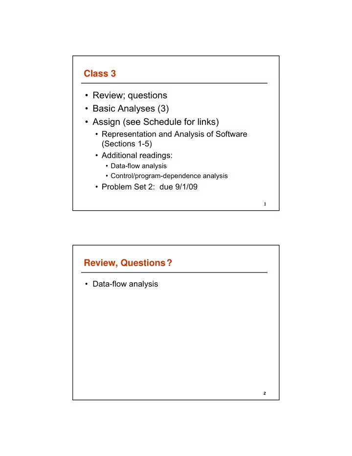
Class 3 • Review; questions • Basic Analyses (3) • Assign (see Schedule for links) • Representation and Analysis of Software (Sections 1-5) • Additional readings: • Data-flow analysis • Control/program-dependence analysis • Problem Set 2: due 9/1/09 1 Review, Questions? • Data-flow analysis 2

Data-flow Analysis 3 3 Introduction (overview) Data-flow analysis provides information for these and other tasks by computing the flow of different types of data to points in the program � For structured programs, data-flow analysis can be performed on an AST; in general, intraprocedural (global) data-flow analysis performed on the CFG � Exact solutions to most problems are undecidable—e.g., � May depend on input � May depend on outcome of a conditional statement � May depend on termination of loop Thus, we compute approximations to the exact solution 4

Introduction (overview) � Approximate analysis can overestimate the solution: � Solution contains actual information plus some spurious information but does not omit any actual information � This type of information is safe or conservative � Approximate analysis can underestimate the solution: � Solution may not contains all information in the actual solution � This type of information in unsafe � For optimization, need safe, conservative analysis � For software engineering tasks, may be able to use unsafe analysis information � Biggest challenge for data-flow analysis: provide safe but precise (i.e., minimize the spurious information) information in an efficient way 5 Introduction (overview) � Approximate analysis can overestimate the solution: � Solution contains actual information plus some spurious information but does not omit any actual information � This type of information is safe or conservative � Approximate analysis can underestimate the solution: � Solution may not contains all information in the actual solution � This type of information in unsafe � For optimization, need safe, conservative analysis � For software engineering tasks, may be able to use unsafe analysis information � Biggest challenge for data-flow analysis: provide safe but precise (i.e., minimize the spurious information) information in an efficient way 6

Introduction (overview) Compute the flow of data to points in the program—e.g., 1. I := 2 � Where does the assignment to I in B1 statement 1 reach? 2. J := I + 1 � Where does the expression computed in statement 2 reach? B2 3. I := 1 � Which uses of variable J are reachable from the end of B1? � Is the value of variable I live after statement 3? B3 4. J := J + 1 Interesting points before and after basic blocks or statements B4 5. J := J - 4 7 Data-flow Problems (reaching definitions) A definition of a variable or memory location is 1. I := 2 a point or statement where that variable gets B1 2. J := I + 1 a value—e.g., input statement, assignment statement. A definition of A reaches a point p if there exists B2 3. I := 1 a control-flow path in the CFG from the definition to p with no other definitions of A on the path (called a definition-clear path) B3 4. J := J + 1 Such a path may exist in the graph but may not be executable (i.e., there may be no input to the program that will cause it to be B4 5. J := J - 4 executed); such a path is infeasible. 8

Data-flow Problems (reaching definitions) � Where are the definitions in the 1. I := 2 program? B1 2. J := I + 1 � Of variable I: � Of variable J: � Which basic blocks (before block) do B2 3. I := 1 these definitions reach? � Def 1 reaches � Def 2 reaches B3 4. J := J + 1 � Def 3 reaches � Def 4 reaches B4 5. J := J - 4 � Def 5 reaches 9 Graph for examples 1. I := 2 B1 2. J := I + 1 B2 3. I := 1 B3 4. J := J + 1 B4 5. J := J - 4 10 10

Data-flow Problems (reaching definitions) � Where are the definitions in the 1. I := 2 program? B1 2. J := I + 1 � Of variable I: 1, 3 � Of variable J: 2, 4, 5 � Which basic blocks (before block) do B2 3. I := 1 these definitions reach? � Def 1 reaches B2 � Def 2 reaches B1, B2, B3 B3 4. J := J + 1 � Def 3 reaches B1, B3, B4 � Def 4 reaches B4 B4 5. J := J - 4 � Def 5 reaches exit 11 11 Iterative Data-flow Analysis (reaching definitions) Method: 1. I := 2 1. Compute two kinds of local information (i.e., B1 within a basic block) 2. J := I + 1 � GEN[B] is the set of definitions that are created (generated) within B � KILL[B] is the set of definitions that, if they B2 3. I := 1 reach the point before B (i.e., the beginning of B) won’t reach the end of B or PRSV[B] is the set of definitions that are preserved (not killed) by B B3 4. J := J + 1 2. Compute two other sets by propagation � IN[B] is the set of definitions that reach the beginning of B; also RCHin[B] B4 5. J := J - 4 � OUT[B] is the set of definitions that reach the end of B; also RCHout[B] 12 12

Iterative Data-flow Analysis (reaching definitions) Method (cont’d): 1. I := 2 B1 3. Propagation method: 2. J := I + 1 � Initialize the IN[B], OUT[B] sets for all B � Iterate over all B until there are no changes to the IN[B], OUT[B] sets B2 3. I := 1 � On each iteration, visit all B, and compute IN[B], OUT[B] as � IN[B] = U OUT[P], P is a B3 4. J := J + 1 predecessor of B � OUT[B] = GEN[B] U (IN[B] ∩ PRSV[B]) B4 5. J := J - 4 or � OUT[B] = GEN[B] U (IN[B] – Kill[B]) 13 13 Iterative Data-flow Analysis (reaching definitions) 1. I := 2 B1 2. J := I + 1 B2 3. I := 1 B3 4. J := J + 1 B4 5. J := J - 4 14 14

Iterative Data-flow Analysis (reaching definitions) Init Init Init Init Iter1 Iter1 Iter2 Iter2 GEN KILL IN OUT IN OUT IN OUT 1 2 3 4 15 15 Iterative Data-flow Analysis (reaching definitions) Data-flow for example (set approach) 1. I := 2 Init Init Init Init Iter1 Iter1 Iter2 Iter2 B1 GEN KILL IN OUT IN OUT IN OUT 2. J := I + 1 1 1,2 3,4,5 -- 1,2 3 1,2 2,3 1,2 B2 3. I := 1 2 3 1 -- 3 1,2 2,3 1,2 2,3 3 4 2,5 -- 4 2,3 3,4 2,3 3,4 B3 4. J := J + 1 4 5 2,4 -- 5 3,4 3,5 3,4 3,5 All entries are sets; sets in red indicate changes B4 5. J := J - 4 from last iteration thus, requiring another iteration of the algorithm 16 16

Iterative Data-flow Analysis (reaching definitions) Data-flow for example (bit-vector approach) 1. I := 2 B1 Init Init Init Init Iter1 Iter1 2. J := I + 1 GEN KILL IN OUT IN OUT 1 B2 3. I := 1 2 3 B3 4. J := J + 1 4 B4 5. J := J - 4 17 Iterative Data-flow Analysis (reaching definitions) Data-flow for example (bit-vector approach) 1. I := 2 B1 Init Init Init Init Iter1 Iter1 2. J := I + 1 GEN KILL IN OUT IN OUT 1 11000 00111 00000 11000 00100 11000 B2 3. I := 1 2 00100 10000 00000 00100 11000 01100 3 00010 01001 00000 00010 01100 00110 B3 4. J := J + 1 4 00001 01010 00000 00001 00110 00101 B4 5. J := J - 4 18

Iterative Data-flow Analysis (reaching definitions) algorithm ReachingDefinitions Input: CFG w/GEN[B], KILL[B] for all B Output: IN[B], OUT[B] for all B Method: Described on slides 17, 18 begin ReachingDefinitions IN[B]=empty; OUT[B]=GEN[B], for all B; change = true while change do begin Change = false foreach B do begin In[B] = union OUT[P], P is a predecessor of B Oldout = OUT[B] OUT[B] = GEN[B] union (IN[B] – Kill[B]) if OUT[B] != Oldout then change = true endfor endwhile end Reaching Definitions 19 Iterative Data-flow Analysis (reaching definitions) Questions about algorithm: 1. Is the algorithm guaranteed to converge? Why or why not? 2. What is the worst-case time complexity of the algorithm? 3. What is the worst-case space complexity of the algorithm? 4. How does depth-first ordering improve the worst-case time complexity? 20

Iterative Data-flow Analysis (reachable uses) A use of a variable or memory location is a 1. I := 2 point or statement where that variable is B1 2. J := I + 1 referenced by not changed --- e.g., used in a computation, used in a conditional, output A use of A is reachable from a point p if there B2 3. I := 1 exists a control-flow path in the CFG from the p to the use with no definitions of A on the path B3 4. J := 1 + J Reachable uses also called upwards exposed uses B4 5. J := J - 4 21 Iterative Data-flow Analysis (reachable uses) � Where are the uses in the 1. I := 2 B1 program? 2. J := I + 1 � Of variable I: 2.1 � Of variable J: 4.2, 5.1 B2 3. I := 1 � From which basic blocks (end of block) are these uses reachable? B3 4. J := 1 + J Use 2.1 is reachable from entry Use 4.2 is reachable from B1, B2, B3 B4 5. J := J - 4 Use 5.1 is reachable from B4 22