CIS 530: Logistic Regression Wrap-up SPEECH AND LANGUAGE PROCESSING - PowerPoint PPT Presentation
CIS 530: Logistic Regression Wrap-up SPEECH AND LANGUAGE PROCESSING (3 RD EDITION DRAFT) CHAPTER 5 LOGISTIC REGRESSION HW 2 is due tonight Leaderboards are before 11:59pm. live until then! Reminders Read Textbook Chapters 3 and 5
CIS 530: Logistic Regression Wrap-up SPEECH AND LANGUAGE PROCESSING (3 RD EDITION DRAFT) CHAPTER 5 “LOGISTIC REGRESSION”
HW 2 is due tonight Leaderboards are before 11:59pm. live until then! Reminders Read Textbook Chapters 3 and 5
Review: Logistic Regression Classifier For binary text classification, consider an input document x , represented by a vector of features [ x 1 , x 2 ,..., x n ]. The classifier output y can be 1 or 0. We want to estimate P ( y = 1| x ) . Logistic regression solves this task by learning a vector of weights and a bias term . 𝑨 = ∑ $ 𝑥 $ 𝑦 $ + 𝑐 We can also write this as a dot product: 𝑨 = 𝑥 ⋅ 𝑦 + 𝑐
Review: Dot product Var Definition Value Weight Product x 1 Count of positive lexicon words 3 2.5 7.5 x 2 Count of negative lexicon words 2 -5.0 -10 x 3 Does no appear? (binary feature) 1 -1.2 -1.2 Num 1 st and 2nd person pronouns x 4 3 0.5 1.5 x 5 Does ! appear? (binary feature) 0 2.0 0 x 6 Log of the word count for the doc 4.15 0.7 2.905 b bias 1 0.1 .1 z=0.805 𝑨 = * 𝑥 $ 𝑦 $ + 𝑐 $
Review: Sigmoid Var Definition Value Weight Product x 1 Count of positive lexicon words 3 2.5 7.5 x 2 Count of negative lexicon words 2 -5.0 -10 x 3 Does no appear? (binary feature) 1 -1.2 -1.2 Num 1 st and 2nd person pronouns x 4 3 0.5 1.5 x 5 Does ! appear? (binary feature) 0 2.0 0 x 6 Log of the word count for the doc 4.15 0.7 2.905 b bias 1 0.1 .1 σ ( 0.805) = 0.69
Review: Learning How do we get the weights of the model? We learn the parameters (weights + bias) via learning. This requires 2 components: 1. An objective function or loss function that tells us distance between the system output and the gold output. We use cross-entropy loss . 2. An algorithm for optimizing the objective function. We will use stochastic gradient descent to minimize the loss function. (We’ll cover SGD later when we get to neural networks).
Re Review: Cross-en entropy lo loss Why does minimizing this negative log probability do what smaller if the model’s we want? We want the lo loss to be sm estimate is cl ct , and we want the lo loss to be close to correct bi bigger er if if it it is is confu fused. It's hokey. There are virtually no surprises , and the writing is second-rate . So why was it so enjoyable? For one thing , the cast is great . Another nice touch is the music . I was overcome with the urge to get off the couch and start dancing . It sucked me in , and it'll do the same to you . P(sentiment=1|It’s hokey...) = 0.69. Let’s say y=1. 𝑧, 𝑧 = −[𝑧 log σ( w · x + b ) + 1 − 𝑧 log(1 − σ( w · x + b ) )] 𝑀 ,- . = −[log σ( w · x + b ) ] = − log ( 0.69 ) = 𝟏. 𝟒𝟖
Re Review: Cross-en entropy l loss ss Why does minimizing this negative log probability do what smaller if the model’s we want? We want the lo loss to be sm estimate is cl ct , and we want the lo loss to be close to correct bi bigger er if if it it is is confu fused. It's hokey. There are virtually no surprises , and the writing is second-rate . So why was it so enjoyable? For one thing , the cast is great . Another nice touch is the music . I was overcome with the urge to get off the couch and start dancing . It sucked me in , and it'll do the same to you . P(sentiment=1|It’s hokey...) = 0.69. Let’s pretend y=0. 𝑧, 𝑧 = −[𝑧 log σ( w · x + b ) + 1 − 𝑧 log(1 − σ( w · x + b ) )] 𝑀 ,- . −[log(1 − σ( w · x + b ) ) ] = − log ( 0.31 ) = 𝟐. 𝟐𝟖 =
Loss on all training examples L 𝑞(𝑧 $ |𝑦 $ ) log 𝑞 𝑢𝑠𝑏𝑗𝑜𝑗𝑜 𝑚𝑏𝑐𝑓𝑚𝑡 = log I $JK L log𝑞(𝑧 $ |𝑦 $ ) = * $JK L 𝑧 $ |𝑧 $ ) = − * L OP (. $JK
Finding good parameters We use gradient descent to find good settings for our weights and bias by minimizing the loss function. L 1 𝑀 ,- (𝑧 $ , 𝑦 $ ; 𝜄) Q 𝜄 = argmin 𝑛 * X $JK Gradient descent is a method that finds a minimum of a function by figuring out in which direction (in the space of the parameters θ) the function’s slope is rising the most steeply, and moving in the opposite direction.
Gradient Descent
CIS 530: Language Modeling with N-Grams SPEECH AND LANGUAGE PROCESSING (3 RD EDITION DRAFT) CHAPTER 3 “LANGUAGE MODELING WITH N- GRAMS”
https://www.youtube.com/watch?v=M8MJFrdfGe0
Autocomplete for texting Machine Translation Probabilistic Language Spelling Correction Models Speech Recognition Other NLG tasks: summarization, question-answering, dialog systems
Goal: compute the probability of a sentence or sequence of words Related task: probability of an upcoming word Probabilistic Language A model that computes either of these is a Modeling language model Better: the grammar But LM is standard in NLP
Goal: compute the probability of a sentence or sequence of words P(W) = P(w 1 ,w 2 ,w 3 ,w 4 ,w 5 …w n ) Related task: probability of an upcoming Probabilistic word P(w 5 |w 1 ,w 2 ,w 3 ,w 4 ) Language Modeling A model that computes either of these P(W) or P(w n |w 1 ,w 2 …w n-1 ) is called a language model . Better: the grammar But language model or LM is standard
How to compute this joint probability: How to ◦ P(the, underdog, Philadelphia, Eagles, won) compute P(W) Intuition: let’s rely on the Chain Rule of Probability
The Chain Rule
The Chain Rule Recall the definition of conditional probabilities p(B|A) = P(A,B)/P(A) Rewriting: P(A,B) = P(A)P(B|A) More variables: P(A,B,C,D) = P(A)P(B|A)P(C|A,B)P(D|A,B,C) The Chain Rule in General P(x 1 ,x 2 ,x 3 ,…,x n ) = P(x 1 )P(x 2 |x 1 )P(x 3 |x 1 ,x 2 )…P(x n |x 1 ,…,x n-1 )
The Chain Rule applied to compute joint probability of words in sentence
The Chain Rule applied to compute joint probability of words in sentence 𝑄 𝑥 K 𝑥 \ ⋯ 𝑥 ^ = I 𝑄(𝑥 $ |𝑥 K 𝑥 \ ⋯ 𝑥 $_K ) $ P(“the underdog Philadelphia Eagles won”) = P(the) × P(underdog|the) × P(Philadelphia|the underdog) × P(Eagles|the underdog Philadelphia) × P(won|the underdog Philadelphia Eagles)
How to estimate these probabilities Could we just count and divide?
How to estimate these probabilities Could we just count and divide? Maximum likelihood estimation (MLE) P(won|the underdog team) = Count(the underdog team won) Count(the underdog team) Why doesn’t this work?
Simplifying Assumption = Markov Assumption
Simplifying Assumption = Markov Assumption P(won|the underdog team) ≈ P(won|team) Only depends on the previous k words, not the whole context ≈ P(won|underdog team) ≈ P(w i |w i-2 w i-1 ) ^ P(w i |w i−k … w i−1 ) P(w 1 w 2 w 3 w 4 …w n ) ≈ ∏ $ K is the number of context words that we take into account
How much history should we use? ^ 𝑞 𝑥 $ = 𝑑𝑝𝑣𝑜𝑢(𝑥 $ ) unigram no history I p( 𝑥 $ ) 𝑏𝑚𝑚 𝑥𝑝𝑠𝑒𝑡 $ ^ 𝑞 𝑥 $ |𝑥 $_K = 𝑑𝑝𝑣𝑜𝑢(𝑥 $_K 𝑥 $ ) bigram 1 word as history I p ( 𝑥 $ |𝑥 $_K ) 𝑑𝑝𝑣𝑜𝑢(𝑥 $_K ) $ ^ trigram 2 words as history 𝑞 𝑥 $ |𝑥 $_\ 𝑥 $_K I p ( 𝑥 $ |𝑥 $_\ 𝑥 $_K ) = 𝑑𝑝𝑣𝑜𝑢(𝑥 $_\ 𝑥 $_K 𝑥 $ ) $ 𝑑𝑝𝑣𝑜𝑢(𝑥 $_\ 𝑥 $_K ) ^ 4-gram 3 words as history 𝑞 𝑥 $ |𝑥 $_h 𝑥 $_\ 𝑥 $_K I p ( 𝑥 $ |𝑥 $_h 𝑥 $_\ 𝑥 $_K ) = 𝑑𝑝𝑣𝑜𝑢(𝑥 $_h 𝑥 $_\ 𝑥 $_K 𝑥 $ ) $ 𝑑𝑝𝑣𝑜𝑢(𝑥 $_h 𝑥 $_h 𝑥 $_K )
Historical Notes 1913 Andrei Markov counts 20k letters in Eugene Onegin 1948 Claude Shannon uses n-grams to approximate English Andrei Markov 1956 Noam Chomsky decries finite-state Markov Models 1980s Fred Jelinek at IBM TJ Watson uses n-grams for ASR, think about 2 other ideas for models: (1) MT, (2) stock market prediction 1993 Jelinek at team develops statistical machine translation 𝑏𝑠𝑛𝑏𝑦 i 𝑞 𝑓 𝑔 = 𝑞 𝑓 𝑞(𝑔|𝑓) Jelinek left IBM to found CLSP at JHU Peter Brown and Robert Mercer move to Renaissance Technology
Simplest case: Unigram model 𝑄 𝑥 K |𝑥 \ ⋯ 𝑥 ^ = I 𝑄(𝑥 $ ) $ Some automatically generated sentences from a unigram model fifth an of futures the an incorporated a a the inflation most dollars quarter in is mass thrift did eighty said hard 'm july bullish that or limited the
Bigram model Condition on the previous word: 𝑄 𝑥 $ |𝑥 K 𝑥 \ ⋯ 𝑥 $_K = 𝑄(𝑥 $ |𝑥 $_K ) texaco rose one in this issue is pursuing growth in a boiler house said mr. gurria mexico 's motion control proposal without permission from five hundred fifty five yen outside new car parking lot of the agreement reached this would be a record november
N-gram models We can extend to trigrams, 4-grams, 5-grams In general this is an insufficient model of language ◦ because language has long-distance dependencies : “The computer(s) which I had just put into the machine room on the fifth floor is (are) crashing.” But we can often get away with N-gram models
Language Modeling ESTIMATING N-GRAM PROBABILITIES
Estimating bigram probabilities The Maximum Likelihood Estimate 𝑄 𝑥 $ 𝑥 $_K = 𝑑𝑝𝑣𝑜𝑢 𝑥 $_K , 𝑥 $ 𝑑𝑝𝑣𝑜𝑢(𝑥 $_K ) 𝑄 𝑥 $ 𝑥 $_K = 𝑑 𝑥 $_K , 𝑥 $ 𝑑(𝑥 $_K )
Recommend
More recommend
Explore More Topics
Stay informed with curated content and fresh updates.
