China, Structural Change, and Multinational Production 1 Kei-Mu Yi - PowerPoint PPT Presentation

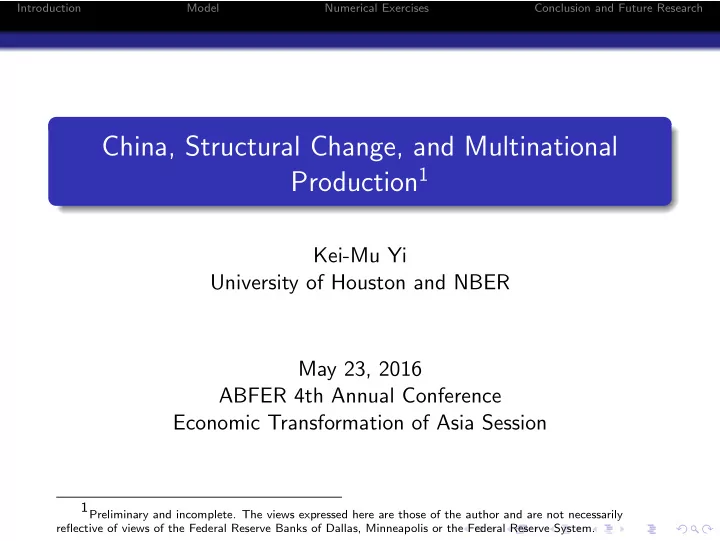
Introduction Model Numerical Exercises Conclusion and Future Research China, Structural Change, and Multinational Production 1 Kei-Mu Yi University of Houston and NBER May 23, 2016 ABFER 4th Annual Conference Economic Transformation of Asia Session 1 Preliminary and incomplete. The views expressed here are those of the author and are not necessarily reflective of views of the Federal Reserve Banks of Dallas, Minneapolis or the Federal Reserve System.

Introduction Model Numerical Exercises Conclusion and Future Research China’s Sectoral Productivity Growth China’s manufacturing (and mining); services (including non-manufacturing industry); and agriculture sectors averaged 8.4, 5.3, and 4.6 percent growth, respectively, in value-added per worker between 1978 and 2010. China sectoral value‐added per worker 90 80 Thousands of 2005 Yuan 70 60 Manufacturing 50 40 30 20 Services 10 Agriculture 0 1960 1970 1980 1990 2000 2010 Data source: GGDC 10-sector database

Introduction Model Numerical Exercises Conclusion and Future Research China’s Trade China Export Share of GDP (percent) 40 35 30 25 20 15 10 5 0 1960 1970 1980 1990 2000 2010 2020 Data source: World Bank, WDI

Introduction Model Numerical Exercises Conclusion and Future Research China’s FDI Inward FDI Stock in Billions of $ U.S. 1995 2011 2012 2013 2014 101.1 711.8 832.9 956.8 1085.3 Source: UNCTAD, World Investment Report 2015

Introduction Model Numerical Exercises Conclusion and Future Research Structural Change in China China Sectoral Employment Shares: 1 0.9 Agriculture 0.8 0.7 0.6 0.5 0.4 Services 0.3 0.2 0.1 Manufacturing 0 1955 1965 1975 1985 1995 2005 2015 Data source: GGDC 10-sector database

Introduction Model Numerical Exercises Conclusion and Future Research Structural Change in United States U.S. Employment Shares: 1 Services 0.8 0.6 0.4 Manufacturing 0.2 Agriculture 0 1950 1954 1958 1962 1966 1970 1974 1978 1982 1986 1990 1994 1998 2002 2006 2010 Data source: GGDC 10-sector database ”Hump” pattern in manufacturing employment shares common in OECD and many EM economies

Introduction Model Numerical Exercises Conclusion and Future Research Structural Change in South Korea 0.8 Agr Man Ser 0.6 Labor Share 0.4 0.2 0 1970 1975 1980 1985 1990 1995 2000 2005 Period Data source: EU KLEMS database

Introduction Model Numerical Exercises Conclusion and Future Research Summary of Preceding Facts China has experienced: High and asymmetric (across sectors) productivity growth Large increase in trade and inward FDI Rapid structural change How do these facts fit together? Before turning to modeling frameworks, a little more data ...

Introduction Model Numerical Exercises Conclusion and Future Research Premature De-Industrialization? Rodrik (2016, JEG) documents: ”A significant deindustrialization trend in recent decades that goes considerably beyond the advanced, post-industrial economies. The hump-shaped relationship between industrialization (measured by employment or output shares) and incomes has shifted downwards and moved closer to the origin. This means countries are running out of industrialization opportunities sooner and at much lower levels of income compared to the experience of early industrializers.”

Introduction Model Numerical Exercises Conclusion and Future Research Trade Openness and Structural Change Structural change is ongoing and evolving in developed and emerging market countries Increased global trade has increased links between developed and emerging market countries Link between globalization and structural change? Autor, Dorn, and Hanson (2012) attribute about 1/4 of decline in U.S. manufacturing employment to trade with China

Introduction Model Numerical Exercises Conclusion and Future Research Manufacturing Trade and Employment Figure: Manufacturing Net Exports and Manufacturing Employment 25% 20% ufacturing Labor Share, 1962 ‐ 2005, 15% TWN MYS KOR THA 10% Percentage Points BOL IDN 5% MEX CRI IND 0% BRA COL PHL PER VEN ‐ 5% PRT ITA JPN CHL FIN ESP ESP Change in Manu CAN CAN ‐ 10% BEL AUT DEN FRA NLD NZL ARG USA ISL NOR ‐ 15% AUS GER SWE CHE ‐ 20% GBR ‐ 25% ‐ 15% ‐ 10% ‐ 5% 0% 5% 10% 15% 20% 25% 30% Change in Manufacturing Net Exports/GDP, 1962 ‐ 2005, Percentage Points

Introduction Model Numerical Exercises Conclusion and Future Research Dominant Frameworks for Modeling Structural Change Non-unitary income elasticity of demand Engel (1895), Kongsamut, Rebelo and Xie (2001) Non-unitary substitution elasticity and sector-biased technical change Baumol (1967), Ngai and Pissarides (2007) Common feature: closed economy frameworks

Introduction Model Numerical Exercises Conclusion and Future Research Recent Research has Highlighted Role of Open Economy in Structural Change Main mechanism involves comparative advantage and international trade Relatively high sectoral productivity growth and/or declines in barriers to trade (trade costs) in a country changes comparative advantage and specialization patterns, which affects sectoral composition of employment (and output) See, for example, Uy, Yi, Zhang (2013); Teignier-Bacque (2014); Sposi (2015); Swiecki (2015); Betts, Giri, Verma (2015) Related research includes Levchenko and Zhang (2016); Caliendo and Parro (2015);

Introduction Model Numerical Exercises Conclusion and Future Research Multinationals and Structural Change Multinationals have played large role in globalization – responsible for significant fraction of increase in international trade, and, most (all?) of increase in FDI Multinationals have played significant role in China’s economic development Boehm, Flaaen, and Pandalai-Nayar (2015) find U.S. multinationals responsible for large share of decline in U.S. manufacturing employment since 1990 What role do multinationals play in hump pattern, and in speeding up of de-industrialization in recent decades?

Introduction Model Numerical Exercises Conclusion and Future Research Goal and What I Do Study role of multinationals in structural change in open economy Develop simple two-country, three-sector model with: Ricardian trade (Eaton and Kortum (2002), Uy, Yi, and Zhang (2013)) Multinational production (Ramondo and Rodriguez-Clare (2013), Alviarez (2014)) Develop intuition for how multinationals can lead to and propagate structural change in an open economy

Introduction Model Numerical Exercises Conclusion and Future Research Set up Two countries Three sectors: agriculture, manufacturing, services Continuum of goods in each sector Services are nontradable One factor of production: labor Mobile across sectors, but immobile across countries Productivity levels (and growth rates) differ across sectors and countries Trade: based on Ricardian comparative advantage Iceberg trade costs Multinational Production: Manufacturing sector only Perfect competition in all markets

Introduction Model Numerical Exercises Conclusion and Future Research Preferences and Budget Constraint Cobb-Douglas utility across sectoral goods: n ) µ a ( C m n ) µ m ( C s n ) µ s U ( C a n , C m n , C s n ) = ( C a Sectoral elasticities of substitution and income: 1 Any change in sectoral labor shares will be because of open economy (trade or MP) CES utility over individual goods: σ � � 1 � σ − 1 σ − 1 C j 0 c j σ du n = n ( u ) Budget constraint (period-by-period): P j n C j ∑ n = w n L n j = a , m , s Static model over time

Introduction Model Numerical Exercises Conclusion and Future Research Technologies Continuum of goods in each sector j : q j n ( u ) = z j n ( u ) L j n ( u ) u ∈ [ 0, 1 ] For j = a , s : z j n ( u ) is distributed as F j n ( z ) = exp ( − T n z − θ ) In manufacturing, there is possibility of multinational production (MP); each country can produce a particular good at home or abroad. Technology is drawn for each production possibility: � � �� li ) − θ F ( z m ∑ ( z m i ; T i ) = exp − T i l Draws are independent of each other Hallmark of MP in model is that home country technology is combined with host country inputs

Introduction Model Numerical Exercises Conclusion and Future Research Input, trade, and MP costs Unit cost of input bundle is: c j n = w n For each sector, iceberg trade costs: d j nl ≥ 1 of sector j goods must be shipped from country l in order for country n to receive one unit For manufacturing, iceberg MP costs, which raise the cost of using technology from country i to produce in country l : c m li = c m l h m li where h m li ≥ 1.

Introduction Model Numerical Exercises Conclusion and Future Research Sectoral Prices (Agriculture and Services) 1 � � 1 � 1 − σ P j 0 p j ( u ) 1 − σ du n = For agriculture (and services), sectoral prices have usual EK formulation: � − 1 / θ � ni ) − θ P a T a i ( c a i d a ∑ n = γ i

Introduction Model Numerical Exercises Conclusion and Future Research Sectoral Prices (Manufacturing; 1) Price that importer country n pays for a manufactured good u is outcome of double minimization: 1 Minimize over host countries for a given technology, e.g., country i technology: ni ( u ) = min l ( c m li d m p m nl li ( ν )) z m Note that there are potentially both MP costs and trade costs 2 Minimize over home country technologies: p m n ( u ) = min i ( p m ni ( u ))