Characterizing the Spatial Variability: examples from the Earth and - PowerPoint PPT Presentation

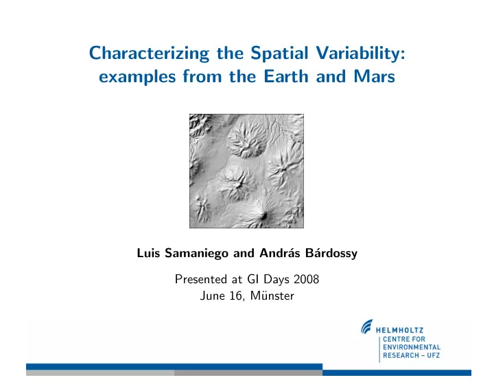
Characterizing the Spatial Variability: examples from the Earth and Mars Luis Samaniego and Andr´ as B´ ardossy Presented at GI Days 2008 June 16, M¨ unster

Outline 1. Motivation 2. Methods to describe the spatial variability 3. Landscape simulations 4. Conclusions 1

Motivation 1. How to analyze the spatial variability of an observable? e.g.: ■ Precipitation ■ Terrain elevation ■ Soil moisture 2

Motivation 1. How to analyze the spatial variability of an observable? e.g.: ■ Precipitation ■ Terrain elevation ■ Soil moisture 2. How to relate it with explanatory variables (i.e. dependence)? 2

Motivation 1. How to analyze the spatial variability of an observable? e.g.: ■ Precipitation ■ Terrain elevation ■ Soil moisture 2. How to relate it with explanatory variables (i.e. dependence)? 3. How to use this knowledge in practical applications? e.g.: ■ Weather generators ■ Simulation / interpolation in Geostatistics 2

Part II Methods to describe the spatial variability

Observable in geophysics z ( x ) = is a realization of a underlining random function Z ( x ) 4

Observable in geophysics z ( x ) = is a realization of a underlining random function Z ( x ) Known: ■ Its variability is a consequence of interactions between natural process ⇒ deterministic ■ Generating processes are sensitive to boundary conditions ■ Exhaustive process description is not possible with known physical/chemical laws 4

Observable in geophysics z ( x ) = is a realization of a underlining random function Z ( x ) Known: ■ Its variability is a consequence of interactions between natural process ⇒ deterministic ■ Generating processes are sensitive to boundary conditions ■ Exhaustive process description is not possible with known physical/chemical laws Unknown: ■ Conditions under which these process took place 4

Observable in geophysics z ( x ) = is a realization of a underlining random function Z ( x ) Known: ■ Its variability is a consequence of interactions between natural process ⇒ deterministic ■ Generating processes are sensitive to boundary conditions ■ Exhaustive process description is not possible with known physical/chemical laws Unknown: ■ Conditions under which these process took place ⇒ Stochastic methods commonly used to extract the spatial dependence 4

Working hypotheses ■ Second order stationarity � Expected value of Z ( x ) E [ Z ( x )] = m � Covariance of two random variables h apart �� �� �� C ( h ) = E Z ( x + h ) − m Z ( x ) − m ■ Intrinsic � Variance of two random variables h apart γ ( h ) = 1 �� � 2 � Z ( x + h ) − Z ( x ) 2 E 5

An example 1 0.8 γ (h) [m²] 0.6 0.4 0.2 0 300 n = 100 000 var(h) x10 3 [m²] 200 100 0 0 10000 20000 30000 h [m] Variogram cloud and experimental variogram from a DEM of the Neckar region (50 × 50) m 6

Shortcomings of the covariance function / variogram ■ Describe the spatial dependence as an integral over the whole range of values 7

Shortcomings of the covariance function / variogram ■ Describe the spatial dependence as an integral over the whole range of values ■ Does not take into account that extremes can have a different spatial dependence structure from the central values (Journel and Alabert, 1989) 7

Shortcomings of the covariance function / variogram ■ Describe the spatial dependence as an integral over the whole range of values ■ Does not take into account that extremes can have a different spatial dependence structure from the central values (Journel and Alabert, 1989) ■ Strongly influenced by the marginal distribution (B´ ardossy, WRR, 2006) 7

Shortcomings of the covariance function / variogram ■ Describe the spatial dependence as an integral over the whole range of values ■ Does not take into account that extremes can have a different spatial dependence structure from the central values (Journel and Alabert, 1989) ■ Strongly influenced by the marginal distribution (B´ ardossy, WRR, 2006) ■ ... What to do? 7

Spatial copula ■ Bivariate distribution function on the unit square with uniform marginals ■ Denotes the pure effect of dependence (Skar 1959, Nelsen 1999) � � � �� � � � � � � � C s ( h , u, v ) = P Z ( x ) < u ; F z Z ( x + h ) = C s Z ( x ) Z ( x + h ) F z < v F z , F z 8

Spatial copula ■ Bivariate distribution function on the unit square with uniform marginals ■ Denotes the pure effect of dependence (Skar 1959, Nelsen 1999) � � � �� � � � � � � � C s ( h , u, v ) = P Z ( x ) < u ; F z Z ( x + h ) = C s Z ( x ) Z ( x + h ) F z < v F z , F z Examples: 1.00 250.00 0.90 100.00 0.80 200.00 90.00 1.15 80.00 0.70 70.00 1.10 0.60 150.00 60.00 1.05 50.00 0.50 1.00 40.00 0.40 100.00 30.00 0.95 20.00 0.30 0.90 10.00 0.20 50.00 0.00 0.85 0.10 0.00 0.00 0.00 0.10 0.20 0.30 0.40 0.50 0.60 0.70 0.80 0.90 1.00 0.00 50.00 100.00 150.00 200.00 250.00 Random field Copula density, h=2 8

Spatial copula ■ Bivariate distribution function on the unit square with uniform marginals ■ Denotes the pure effect of dependence (Skar 1959, Nelsen 1999) � � � �� � � � � � � � C s ( h , u, v ) = P Z ( x ) < u ; F z Z ( x + h ) = C s Z ( x ) Z ( x + h ) F z < v F z , F z Examples: 1.00 250 0.90 0.04 0.80 200 10.00 9.00 0.03 0.70 8.00 0.60 150 7.00 6.00 0.02 0.50 5.00 4.00 100 0.40 3.00 0.01 0.30 2.00 1.00 50 0.20 0.00 0.00 0.10 0 0.00 0 50 100 150 200 250 0.00 0.10 0.20 0.30 0.40 0.50 0.60 0.70 0.80 0.90 1.00 Normal field Copula density, h=4 8

Estimation of an empirical copula Step 1 : Select a spatial domain, e.g. a DEM. 50 20 80 100 80 90 50 25 10 60 0 30 20 40 10 5 DEM 9

Estimation of an empirical copula Step 2 : Estimate its empirical distribution function F n ( z ) . Empirical Distribution Function of z 1 0.8 0.6 F(z) 0.4 0.2 0 0 25 50 75 100 z 50 20 80 100 80 90 50 25 10 60 0 30 20 5 40 10 DEM 10

Estimation of an empirical copula Step 3 : Built a grid having the corresponding F n ( z ) values. Empirical Distribution Function of z 1 0.8 0.6 F(z) 0.4 0.2 0 0 25 50 75 100 z 0.38 0. 69 0 .8 8 1 .00 50 20 80 100 0.94 0.88 0.69 0.44 80 90 50 25 0.06 0.25 0.50 0.75 10 60 0 30 0.56 0.38 0.25 0.13 20 5 40 10 Marginal d istribution DEM of the DEM 11

Estimation of an empirical copula Step 4 : Sample N pairs from it: ( u = F n ( z ) , v = F n ( z + h )) 0.38 0.69 0.88 1.00 0.94 0.88 0.69 0.44 0.06 0.25 0.50 0.75 0.56 0.38 0.25 0.13 Marginal d istribution of the DEM 12

Estimation of an empirical copula Step 5 : Store all pairs ( u, v ) and ( v, u ) . Tally the frequencies 1 0.38 0.69 0.88 1.00 0.8 0.94 0.88 0.69 0.44 0.6 v 0.4 0.06 0.25 0.50 0.75 0.2 0.56 0.38 0.25 0.13 0 0 0.2 0.4 0.6 0.8 1 u Marginal d istribution of the DEM 13

Estimation of an empirical copula Step 6 : Normalize both marginals and calculate the copula density c s ( u, v ) . 1 0.38 0.69 0.88 1.00 0.8 0.94 0.88 0.69 0.44 0.6 v 0.4 0.06 0.25 0.50 0.75 0.2 0.56 0.38 0.25 0.13 0 0 0.2 0.4 0.6 0.8 1 u Marginal d istribution of the DEM Σ = 1 1 Σ = 1 0.8 4 0.6 3 v 2 0.4 1 0 0.2 0 0 0.2 0.4 0.6 0.8 1 u E. copula density h=1 14

Part II Examples

Variation of the spatial dependency with h ~ 5 km 1 10.5 0.8 9 7 0.6 5 v 4 0.4 3 2 1 0.2 0 0 0 0.2 0.4 0.6 0.8 1 Andean landscape u 3 h = ~ 1.0 km Disorder r = ~ 0.97 2 E 1 Order 0 0.2 0.4 0.6 0.8 1 u 16

Variation of the spatial dependency with h ~ 5 km 1 10.5 0.8 9 7 0.6 5 v 4 0.4 3 2 1 0.2 0 0 0 0.2 0.4 0.6 0.8 1 Andean landscape u 3 h = ~ 2.5 km Disorder r = ~ 0.89 2 E 1 Order 0 0.2 0.4 0.6 0.8 1 u 17

Variation of the spatial dependency with h ~ 5 km 1 10.5 0.8 9 7 0.6 5 v 4 0.4 3 2 1 0.2 0 0 0 0.2 0.4 0.6 0.8 1 Andean landscape u 3 h = ~ 5.0 km Disorder r = ~ 0.69 2 E 1 Order 0 0.2 0.4 0.6 0.8 1 u 18

Relation of the spatial copula and the geomorphologic genesis ~ 120 km 1 10.5 0.8 8 0.6 v 5 0.4 2 0.2 0 0 0 0.2 0.4 0.6 0.8 1 u Xanthe Terra (Mars) h = ~ 20 km r = ~ 0.89 19

Relation of the spatial copula and the geomorphologic genesis ~ 5 km 1 10.5 9 0.8 7.5 0.6 6 v 4.5 0.4 3 0.2 1.5 0 0 0 0.2 0.4 0.6 0.8 1 u Cotopaxi Volcano (Ecuador) h = ~ 2.5 km r = ~ 0.88 20

Relation of the spatial copula and the geomorphologic genesis ~ 2 km 1 10.5 9 0.8 7.5 0.6 6 v 4.5 0.4 3 0.2 1.5 0 0 0 0.2 0.4 0.6 0.8 1 u Headwater Neckar (Germany) h = ~ 1.00 km r = ~ 0.86 21

Relation of the spatial copula and the geomorphologic genesis ~ 10 km 1 10.5 9 0.8 7.5 0.6 6 v 4.5 0.4 3 0.2 1.5 0 0 0 0.2 0.4 0.6 0.8 1 u Marzuq Desert (Libya) h = ~ 0.36 km r = ~ 0.89 22

Shannon’s entropy of the spatial copulas � E ( u ) = − c s ( u, u 2 ) log c s ( u, u 2 ) du 2 (1) u 2 Neckar Disorder Cotopaxi 3 Sahara Xanthe Terra (Mars) Random field Gaussian field 2 E 1 Order 0 0 0.2 0.4 0.6 0.8 1 u 23

Part III Landscape simulations