Characterizing extremal limits Oleg Pikhurko University of Warwick - PowerPoint PPT Presentation
Characterizing extremal limits Oleg Pikhurko University of Warwick ICERM, 11 February 2015 Rademacher Problem g ( n , m ) := min { # K 3 ( G ) : v ( G ) = n , e ( G ) = m } Mantel 1906, Turn41: max { m : g ( n , m ) = 0 } = n 2
Characterizing extremal limits Oleg Pikhurko University of Warwick ICERM, 11 February 2015
Rademacher Problem ◮ g ( n , m ) := min { # K 3 ( G ) : v ( G ) = n , e ( G ) = m } ◮ Mantel 1906, Turán’41: max { m : g ( n , m ) = 0 } = ⌊ n 2 4 ⌋ ◮ Rademacher’41: g ( n , ⌊ n 2 4 ⌋ + 1 ) = ⌊ n 2 ⌋
Just Above the Turán Function os’55: m ≤ ⌊ n 2 ◮ Erd˝ 4 ⌋ + 3 os’62: m ≤ ⌊ n 2 ◮ Erd˝ 4 ⌋ + ε n os’55: Is g ( n , ⌊ n 2 4 ⌋ + q ) = q · ⌊ n ◮ Erd˝ 2 ⌋ for q < n / 2 ? ◮ K k , k + q edges versus K k + 1 , k − 1 + ( q + 1 ) edges ◮ Lovász-Simonovits’75: Yes ◮ Lovász-Simonovits’83: m ≤ ⌊ n 2 4 ⌋ + ε n 2
Asymptotic Version g ( n , a ( n 2 ) ) ◮ g ( a ) := lim n →∞ ( n 3 ) ◮ Upper bound: K cn ,..., cn , ( 1 − tc ) n ◮ Moon-Moser’62,Nordhaus-Stewart’62 (Goodman’59): g ( a ) ≥ 2 a 2 − a ◮ Bollobás’76: better lower bound ◮ Fisher’89: g ( a ) for 1 2 ≤ a ≤ 2 3 ◮ Razborov’08: g ( a ) for all a ◮ No stability ◮ H a n : modify the last two parts of K cn ,..., cn , ( 1 − tc ) n ◮ P .-Razborov ≥ ’15: ∀ almost extremal G n is o ( n 2 ) -close to some H a n
Possible Edge/Triangle Densities K 3 K 3 1.0 1.0 0.8 0.8 0.6 0.6 0.4 0.4 0.2 0.2 K 2 0.2 0.4 0.6 0.8 1.0 K 2 0.2 0.4 0.6 0.8 1.0 ◮ Upper bound: Kruskal’63, Katona’66
Limit Object ◮ Subgraph density G [ random v ( F ) -set ] ∼ � � p ( F , G ) = Prob = F ◮ F 0 = { finite graphs } ◮ ( G n ) converges if v ( G n ) → ∞ and ∀ F ∈ F 0 ∃ lim n →∞ p ( F , G n ) =: φ ( F ) ◮ LIM = { all such φ } ⊆ [ 0 , 1 ] F 0 ◮ g ( a ) = inf { φ ( K 3 ) : φ ∈ LIM , φ ( K 2 ) = a }
Razborov’s Flag Algebra A 0 ◮ φ ∈ LIM ⊆ [ 0 , 1 ] F 0 ◮ F 0 = { unlabeled graphs } ◮ R F 0 := { quantum graphs } = { � α i F i } ◮ Linearity: φ : R F 0 → R ◮ A 0 := R F 0 / � � linear relations that always hold ◮ φ ( F 1 ) φ ( F 2 ) = � c H φ ( H ) ◮ Define: F 1 · F 2 := � H c H H ◮ φ : A 0 → R is algebra homomorphism
Positive Homomorphisms ◮ φ ∈ Hom ( A 0 , R ) is positive if ∀ F ∈ F 0 φ ( F ) ≥ 0 ◮ Hom + ( A 0 , R ) = { positive homomorphisms } ◮ Lovász-Szegedy’06, Razborov’07: LIM = Hom + ( A 0 , R ) ◮ ⊇ : Let φ ∈ Hom + ( A 0 , R ) ◮ � | F | = n φ ( F ) = 1 ◮ Distribution on F 0 n ◮ Prob [ random G n → φ ] = 1 ◮ φ ∈ LIM ◮ Write � α i F i ≥ 0 if ◮ ∀ φ ∈ Hom + ( A 0 , R ) � α i φ ( F i ) ≥ 0 lim inf � α i p ( F i , G n ) ≥ 0 ◮ Equivalently: ∀ ( G n )
Limit version of the problem ◮ g ( a ) = min { φ ( K 3 ) : φ ∈ Hom + ( A 0 , R ) , φ ( K 2 ) = a } ◮ Characterise all extremal φ : { φ ∈ Hom + ( A 0 , R ) : φ ( K 3 ) = g ( φ ( K 2 )) } = ? ◮ Alternatively: work with graphons. E.g. g ( a ) = min { t ( K 3 , W ) : graphon W with t ( K 2 , W ) = a }
Razborov’s Proof for a ∈ [ 1 2 , 2 3 ] ◮ h ( a ) = conjectured value ◮ Hom + ( A 0 , R ) ⊆ [ 0 , 1 ] F is closed ⇒ compact ◮ f ( φ ) := φ ( K 3 ) − h ( φ ( K 2 )) is continuous ◮ ∃ φ 0 that minimises f on { φ ∈ Hom + ( A 0 , R ) : 1 2 ≤ φ ( K 2 ) ≤ 2 3 } ◮ a := φ 0 ( K 2 ) � n ◮ c : e ( K cn , cn , ( 1 − 2 c ) n ) ≈ a � 2
Goodman bound ◮ Goodman bound: K 3 − K 2 ( 2 K 2 − 1 ) ≥ 0 ◮ Cauchy-Schwarz: [ [ K 1 2 · K 1 2 ] ] 1 ≥ K 2 · K 2 6 ¯ ◮ [ [ K 1 2 · K 1 ] 1 = 1 2 K 3 + 1 2 K 2 − 1 P 3 ≤ 1 2 K 3 + 1 2 ] 2 K 2 ◮ Assume 1 2 < a < 2 3 ◮ Otherwise done by the Goodman bound ◮ h is differentiable at a
At Most cn Triangles per Edge ◮ Pick G n → φ 0 ◮ Rate of growth: g ( n , m + 1 ) − g ( n , m ) ≈ cn ◮ ≈ cn triangles per new edge ◮ G n has � cn triangles on almost every edge ◮ Flag algebra statement φ E 0 ( K E 3 ) ≤ c a.s. ◮ Informal explanation: ◮ φ E 0 : Two random adjacent roots x 1 , x 2 in G n ◮ K E 3 : Density of rooted triangles
Flag Algebra A E ◮ E := ( K 2 , 2 roots ) ◮ F E := { ( F , x 1 , x 2 ) : F ∈ F 0 , x 1 ∼ x 2 } ◮ p ( F , G ) : root-preserving induced density ◮ G n ∈ F E converges if ∀ F ∈ F E p E ( F , G n ) → φ E ( F ) ◮ φ E : R F E → R ◮ A E := � R F E / � trivial relations � , multiplication � ◮ Razborov’07: { limits φ E } = Hom + ( A E , R ) ◮ Random homomorphism φ E 0 ( K E 3 ) : ◮ G n → φ ◮ ( G n , [random x 1 ∼ x 2 ] ) ∈ M ( F E ) ◮ Weak limit
Vertex Removal ◮ Remove x ∈ V ( G n ) : ◮ ∂ p ( K 2 , G n ) : ◮ Remove edges: − d ( x ) �� n � 2 � n ��� n − 1 ◮ Remove isolated x : × = 1 + 2 � n + ... 2 2 ◮ Total change: − K 1 � n + a 2 � 2 ( x ) / n + ... 2 � n ◮ ∂ p ( K 3 , G n ) = − K 1 + φ 0 ( K 3 ) 3 � 3 ( x ) / n + ... 3 ◮ Expect: ∂ p ( K 3 ) � h ′ ( a ) ∂ p ( K 2 ) ◮ Cloning x: signs change ◮ Approximate equality for almost all x ◮ Flag algebra statement: − 3 ! φ 1 0 ( K 1 − 2 φ 1 0 ( K 1 � � 3 ) + 3 φ 0 ( K 3 ) = 3 c 2 ) + 2 a a . s .
Finishing line ◮ Recall: A.s. ◮ − 3 ! φ 1 0 ( K 1 � − 2 φ 1 0 ( K 1 � 3 ) + 3 φ 0 ( K 3 ) = 3 c 2 ) + 2 a 0 ( K E ◮ φ E 3 ) ≤ c ◮ Average? ◮ 0 = 0 � ◮ Slack � E ◮ Multiply by K 1 2 & P 3 and then average! ◮ Calculations give φ 0 ( K 3 ) ≥ 3 ac ( 2 a − 1 ) + φ 0 ( K 4 ) + 1 4 φ 0 ( K 1 , 3 ) 3 c + 3 a − 2 φ 0 ( K 3 ) ≥ h ( a ) � ◮ φ 0 ( K 4 ) ≥ 0 & φ 0 ( K 1 , 3 ) ≥ 0 ⇒
Extremal Limits ◮ Extremal limit: limits of almost extremal graphs ◮ Equivalently: { φ ∈ Hom + ( A 0 , R ) : φ ( K 3 ) = g ( φ ( K 2 )) } ◮ P .-Razborov ≥ ’15: { extremal limits } = { limits of H a n ’s } ◮ Implies the discrete theorem ◮ Pick a counterexample ( G n ) ◮ Subsequence convergent to some φ ◮ H a n → φ ◮ δ � ( G n , H a n ) → 0 ◮ Overlay V ( G n ) = V ( H a n ) = V 1 ∪ · · · ∪ V t − 1 ∪ U ◮ G [ V i , V i ] almost complete ◮ G [ V i ] almost empty ◮ G [ U ] has o ( n 3 ) triangles
Structure of Extremal φ 0 ◮ Assume φ 0 ( K 3 ) = h ( a ) ( = g ( a ) ) with 1 2 ≤ a ≤ 2 3 ◮ If a ∈ { 1 2 , 2 3 } : ◮ Goodman’s bound is sharp ◮ φ 0 (¯ P 3 ) = 0 ◮ Complete partite ◮ Cauchy-Schwarz ⇒ regular ◮ φ 0 is the balanced k -partite limit, done! � ◮ Suppose a ∈ ( 1 2 , 2 3 ) ◮ Density of K 4 and K 1 , 3 is 0 ◮ If φ 0 ( P 3 ) = 0, ◮ Complete partite ◮ K 4 -free ⇒ at most 3 parts ⇒ done! �
Case 2: φ 0 ( P 3 ) > 0 ◮ Special graphs F 1 and F 2 : ◮ Claim: φ 0 ( F 1 ) = φ 0 ( F 2 ) = 0 ◮ Claim: Exist many P 3 ’s st ◮ | A | = Ω( n ) : vertices sending 3 edges to it ◮ | B | = Ω( n ) : vertices sending ≤ 2 edges to it ◮ Non-edge across → a copy of F 1 , F 2 , or K 1 , 3 ◮ G n [ A , B ] is almost complete ⇒ � ◮ K 4 -freeness + calculations
Clique Minimisation Problem ◮ Open: Exact result for K 3 ◮ Nikiforov’11: Asymptotic solution for K 4 ◮ Reiher ≥ ’15: Asymptotic solution for K r ◮ Open: Structure & exact result
General Graphs ◮ Colour critical: χ ( F ) = r + 1 & χ ( F − e ) = r ◮ Simonovits’68: ex ( n , F ) = ex ( n , K r + 1 ) , n ≥ n 0 ◮ Mubayi’10: Asymptotic for m ≤ ex ( n , F ) + ε F n ◮ P .-Yilma ≥ ’15: Asymptotic for m ≤ ex ( n , F ) + o ( n 2 ) ◮ Bipartite F ◮ Conjecture (Erd˝ os-Simonovits’82, Sidorenko’93): ◮ Random graphs are optimal ◮ ..., Conlon-Fox-Sudakov’10, Li-Szegedy ≥ ’15, Kim-Lee-Lee ≥ ’15, ... ◮ Forcing Conjecture (Li-Szegedy): F biparite non-tree ⇒ extremal graphons are constants
Thank you!
Recommend
More recommend
Explore More Topics
Stay informed with curated content and fresh updates.

