Chapter 8 Hypothesis Testing Chapter problem: Does the MicroSort - - PowerPoint PPT Presentation

1

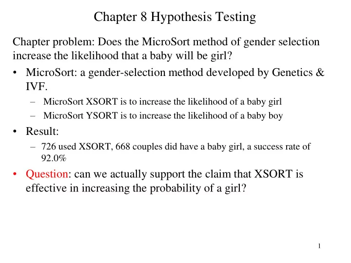
Chapter 8 Hypothesis Testing

Chapter problem: Does the MicroSort method of gender selection increase the likelihood that a baby will be girl?

• MicroSort: a gender-selection method developed by Genetics &

IVF.

– MicroSort XSORT is to increase the likelihood of a baby girl – MicroSort YSORT is to increase the likelihood of a baby boy

• Result:

– 726 used XSORT, 668 couples did have a baby girl, a success rate of 92.0%

• Question: can we actually support the claim that XSORT is

effective in increasing the probability of a girl?

2

8.1 Overview

Definition – In statistics, a hypothesis is a claim or statement about a property of a population. A hypothesis test (or test of significance) is a standard procedure for testing a claim about a property of a population. Examples: Genetics, Business, Medicine, Aircraft Safety, Quality Control. Rare Event Rule for Inferential Statistics: If, under a given assumption, the probability of a particular

• bserved event is extremely small, we conclude that the

assumption is probably not correct.

3

8.1 Overview

e.g.1 Gender Selection. A product named “Gender Choice”

• The Ad claims “increase your chances of having a girl up to 80%”
• Assumption: Gender Choice had no effect
• If 100 couples using Gender Choice have 100 babies

a. Consisting of 52 girls b. Consisting of 97 girls

• What should we conclude about the assumption?

Sol.

• a. There is no sufficient evidence that Gender Choice is effective

(common sense) (52 out of 100 is not significant)

• b. Explained it in two ways. One explanation is that extremely

rare event happened. The other is that the assumption is not true, i.e. Gender Choice is effective. (97 out of 100 is significant)

4

8.2 Basics of Hypothesis Testing

Key Concept

• Null hypothesis
• Alternative hypothesis
• Test statistics
• Critical region
• Significance level
• Critical value
• P-value
• Type-I error
• Type-II error

5

8.2 Basics of Hypothesis Testing – Part I

Objective for Part I

• Given a claim, identify the null hypothesis and alternative

hypothesis, express them in symbolic form

• Given a claim and sample data, calculate the value of the test

statistics

• Given a significance level, identify the Critical value(s).
• Given a value of the test statistic, identify the P-value
• State the conclusion of a hypothesis test in simple, non-technical

terms.

6

8.2 Basics of Hypothesis Testing – Part I

Need to understand this example (show concept and process) e.g.2 Chapter problem (continue). Key points:

• Claim: for couples using XSORT, the proportion of girls is p > 0.5
• Working assumption: The proportion of girls is p = 0.5 (with no effect

from XSORT)

• The sample resulted in 13 girls among 14 births, so the sample

proportion is = 13/14 = 0.929.

• Assuming that p = 0.5, P(13 girls or more in 14 births) = 0.0016.
• Two possible explanations for the results of 13 girls in 14 births:

– either the random chance event (with prob. 0.0016) has occurred, – or the proportion of girls born to couple using Gender Choice is greater than 0.5.

• Because the random chance is so small, we reject the random chance

and conclude that there is sufficient evidence to support a claim that XSORT is effective.

p ˆ

7

8.2 Basics of Hypothesis Testing – Part I

Working with the Stated Claim: Null and Alternative Hypothesis

• The Null hypothesis (denoted by H0) is that the parameter (e.g. proportion,

mean, and SD) equal to some claim value. E.g. H0: p = 0.5, H0:  = 98.6, H0:  = 15,

• The Alternative hypothesis (denoted by H1) is that the parameter has a value

that differs from the one in null hypothesis. Proportions H1: p > 0.5, H1: p < 0.5, H1: p  0.5, means: H1:  > 98.6, H1:  < 98.6, H1:   98.6, SD’s: H1:  > 15, H1:  < 15, H1:   15,

• Always use equal symbol in null hypothesis H0.

8

8.2 Basics of Hypothesis Testing – Part I

Working with the Stated Claim: Null and Alternative Hypothesis Procedure of Identifying the null and alternative hypothesis

start Identify the specific claim or hypothesis to be tested, and express it in symbolic form Give the symbolic form that must be true when the original is false Of the two symbolic expressions obtained so far, let the alternative hypothesis H1uses the symbol < or > or . Let the null hypothesis H0 be the symbolic expression that the parameter equals the fixed value being considered.

Figure 8.2 Identifying

H0 and H1

9

8.2 Basics of Hypothesis Testing – Part I

Working with the Stated Claim: Null and Alternative Hypothesis e.g.3 Identifying the Null and Alternative hypotheses. Claim: the mean weight of airline passengers (including carry on baggage) is at most 195 pounds.

• Sol. Following Figure 8-2.

Step 1.   195. (translate “mean weight … is at most 195 lbs”) Step 2. If p ≤ 195 is false, then  > 195 Step 3. Therefore we determine H0 and H1, H1:  > 195, and H0:  = 195

10

8.2 Basics of Hypothesis Testing – Part I

Converting Sample Data to a Test Statistic Test statistic for proportion Test statistic for mean or Test statistic for SD

n pq

p p z   ˆ

n

x z



  

n s

x t   

2 2 2

) 1 (   s n  

11

8.2 Basics of Hypothesis Testing – Part I

Converting Sample Data to a Test Statistic

e.g.4 Finding the Test Statistic. Claim: XSORT increase the likelihood of having a baby girl. Preliminary results from a test of the XSORT involved 14 couples who gave birth to 13 girls and 1 boy. Use the given claim and the preliminary results to calculate the value of the test statistic. Use the format given, so that a normal distribution is used to approximate a binomial distribution.

• Sol. H0: p = 0.5,

H1: p > 0.5, test statistic: Interpretation: z score of 3.21 is unusual. It fall within the range

• f values considered to be significant because they are so far

above 0.5 that they are not likely to occur by chance. (see graph in next page)

21 . 3 5 . 929 . ˆ

14 ) 5 . )( 5 . (

    

n pq

p p z

12

8.2 Basics of Hypothesis Testing – Part I

My comment: this is a right tail test.

Sample proportion of:

• r

Test Statistic z = 3.21

ˆ p  0.929

Figure 8-3 Critical Region, Critical Value, Test Statistic

13

8.2 Basics of Hypothesis Testing – Part I

Tools for Assessing the Test Statistic: Critical Region, Significant Level, Critical Value, and P-Value

• The critical region (or rejection region) is the set of all values of

the test statistics that cause us to reject the null hypothesis. For example, Figure 8-3

• The significant level (denoted by , the same  introduce in 7.2)

is the probability that the test statistic will fall in the critical region when the null hypothesis is actually true. If the test statistic fall into the critical region, we reject the null hypothesis.

• The critical value is any value that separates the critical region

from the values of the test statistic that do not lead to rejection of the null hypothesis.

14

8.2 Basics of Hypothesis Testing – Part I

e.g.5 and e.g.6 Finding Critical Values. Using the significance level of

 = 0.05, find the critical z values for each of the following alternative

• hypothesis. (Assuming normal distribution can be used to approximate the

binomial distribution):

a. H1: p  0.5 b. H1: p < 0.5 c. H1: p > 0.5

• Sol. Draw Figure 8–4 on the blackboard.
• By examining the alternative hypothesis, we can determine

whether a test is right-tailed (H1: > ), left-tailed (H1: < ) or two-

• tailed. (Draw Figure 8-6).
• The tail corresponds to the critical region containing the values

that would conflict significantly with the null hypothesis.

15

8.2 Basics of Hypothesis Testing – Part I

The P-Value (or probability value) is the probability of getting a value of the test statistic that is at least as extreme as the one representing the sample data, assume that the null hypothesis is

• true. (next page, Figure 8 – 5) P-value can be found after

finding the area in Figure 8-5.

16

8.2 Basics of Hypothesis Testing – Part I

Decisions and Conclusions The standard procedure of hypothesis testing requires that we always test the null hypothesis first. So the initial conclusion will be one of the following:

– Reject the null hypothesis – Fail to reject the null hypothesis

A memory tool useful for interpreting the P-values:

– If the P is low, the null must go. – If the P is high, the null will fly.

17

8.2 Basics of Hypothesis Testing – Part I

Decisions and Conclusions

start

What Type of test ?

Is the test statistic to the right or left of Center ?

Left-tailed Right-tailed Two-tailed Left Right

P-Value = area to the left of the test statistics P-Value = Twice the area to the left

• f the test statistics

P-Value = Twice the area to the right

• f the test statistics

P-Value = area to the right of the test statistics

Figure 8 – 5 Procedure for Finding P-values Draw 4 pictures in class accordingly.

18

8.2 Basics of Hypothesis Testing – Part I

Decisions and Conclusions

Decision Criterion:

– Traditional method: reject H0 if test statistic falls within the critical

• region. Fail to reject H0 if test statistic does not fall within the critical

region – P-Value method: reject H0 if P-value   (where  is the significance level, such as 0.05). Fail to reject H0 if P-value > . – Another option: instead of using the significance level, simply identify P-value and leave the decision to the reader. – CI method: because a CI estimate of a population parameter contains the likely values of that parameter, reject a claim that the population parameter has a value that is not included in CI.

19

8.2 Basics of Hypothesis Testing – Part I

Decisions and Conclusions

e.g.7 Finding P-Values for a Critical Region in the Right Tail. Claim: XSORT increase the likelihood of having a baby girl. Preliminary results from a test of the XSORT involved 14 couples who gave birth to 13 girls and 1 boy. Find P-Value, and interpret the P-value

• Sol. Consider H1 : p > 0.5. z = 3.21 (e.g.4), area to the right of z =

3.21 is 0.0007. So P-value = 0.0007. Interpretation: P = 0.0007, it shows that there is very small chance of getting the sample result that led to a test statistic z = 3.21. It is very unlikely that we will get 13 (or more) girls in 14 births by

• chance. This suggest that XSORT is effective for gender

selection.

20

8.2 Basics of Hypothesis Testing – Part I

Decisions and Conclusions

e.g.8 Finding P-Values for a Critical Region in two tails. Claim: with the XSORT, the likelihood of having a baby girl is different from p = 0.5. Preliminary results from a test of the XSORT involved 14 couples who gave birth to 13 girls and 1 boy. Find P-Value, and interpret the P-value. (same problem like e.g.7, H1 changed)

• Sol. Consider H1 : p  0.5. z = 3.21 (e.g.4), area to the right of z =

3.21 is 0.0007. So P-value = 2(0.0007) = 0.0014. Interpretation: P = 0.0014, it shows that there is very small chance of getting the sample result that led to a test statistic z = 3.21. It is very unlikely that we will get 13 (or more) girls in 14 births by

• chance. This suggest that with XSORT, the likelihood of

having a baby girl is different from 0.5.

21

8.2 Basics of Hypothesis Testing – Part I

Decisions and Conclusions Wording the Final Conclusion.

start

Does the Original claim contain The condition of Equality?

yes no

Do you Reject H0? Do you Reject H0?

Original claim contains equality Original claim does not contains Equality and becomes H1 Yes, reject H0 No, Fail to reject H0 No, Fail to reject H0 Yes, reject H0

There is sufficient evidence to warrant rejection of the claim that … (original claim) There is not sufficient evidence to warrant rejection of the claim that … (original claim) The sample data support the claim that … (original claim) There is not sufficient sample evidence to support the claim that … (original claim) (this is the only case in which the original claim is rejected) (this is the only case in which the original claim is supported)

Figure 8 – 7 Wording of Final Conclusion

22

8.2 Basics of Hypothesis Testing – Part I

Wording the Final Conclusion e.g.9 Stating the Final Conclusion.

–

• XSORT. 13 Girls in 14 birth after using XSORT.

– H1: p > 0.5, H0: p = 0.5 – P-Value = 0.0007 – reject the null hypothesis of p = 0.5.

State the conclusion in simple non-technical terms. Ans: by Figure 8 – 7, the conclusion is as simple as follows: “The sample data support the claim that the XSORT method of gender selection increases the likelihood of a baby girl”

23

8.2 Basics of Hypothesis Testing – Part I

Errors in Hypothesis Tests Type I and Type II Errors True State of Nature

The null hypothesis is true The null hypothesis is false We decide to reject the null hypothesis Type I error (rejecting a true null hypothesis)  Correct Decision We fail to reject the null hypothesis Correct Decision Type II error (Failing to reject a false null hypothesis) 

Decision

Table 8 – 1 Type I and Type II errors

24

8.2 Basics of Hypothesis Testing – Part I

Errors in Hypothesis Tests Notation  (alpha) = probability of a type I error (the probability of rejecting H0 when it is true)  (beta) = probability of a type II error (the probability of failing to reject H0 when it is false) e.g.10 XSORT. H1 : p > 0.5. Claim: XSORT increase the likelihood

• f a baby girl.

a. Type I error is made when XSORT has no effect, we conclude that XSORT is effective. b. Type II error is made when XSORT is effective, we conclude that XSORT has no effect.

25

8.2 Basics of Hypothesis Testing – Part I

Comments

• Don’t use “Accept” for “Fail to Reject”
• Don’t use Multiple Negatives

Comprehensive Hypothesis Test

• Details of P-value method, traditional method, and CI method
• Next three pages (examples in next section)

26

8.2 Basics of Hypothesis Testing – Part I

P-Value Method

Step 1. Identify the specific claims and put it in symbolic form Step 2. Give the symbolic form that must be true when the original claim is false Step 3. Obtain H1 and H0 Step 4. Select the significance level  based on the seriousness of a type I error. make  small if consequences of rejecting a true H0 are severe. (for example 0.05 and 0.01) Step 5. Identify the statistic (such as normal, t, chi-square). Step 6. Find the test statistic and find the P-value (see Figure 8 – 6, page 16). Draw a graph and show the test statistic and P-value Step 7. Reject H0 if the P-value is less than or equal to the significance level . Fail to reject H0 if the P-value is greater than . Step 8. Restate this previous decision in simple, non-technical terms, and address the original claim.

27

8.2 Basics of Hypothesis Testing – Part I

Traditional Method

Step 1. Identify the specific claims and put it in symbolic form Step 2. Give the symbolic form that must be true when the original claim is false Step 3. Obtain H1 and H0 Step 4. Select the significance level  based on the seriousness of a type I error. make  small if consequences of rejecting a true H0 are severe. (for example 0.05 and 0.01) Step 5. Identify the statistic (such as normal, t, chi-square). Step 6. Find the test statistic, the critical values and the critical region. Draw a graph Step 7. Reject H0 if test statistic is in the critical region. Fail to reject H0 if the test statistic is not in the critical region. Step 8. Restate this previous decision in simple, non-technical terms, and address the original claim.

28

8.2 Basics of Hypothesis Testing – Part I

Confidence Method

• Construct a CI with a confidence level selected as in Table 8–2
• Because a CI estimate of a population parameter contains the

likely values of that parameter, reject a claim that the population parameter has a value that is not included in the CI.

• For one-tail hypothesis test with significance level , construct a

CI with CL of 1 – 2. See Table 8-2 Two-Tailed Test One-Tailed Test Significance 0.01 99% 98% Levels for 0.05 95% 90% Hypothesis 0.10 90% 80% Test Table 8-2 CL for CI

29

8.3 Testing a Claim About a Proportion

• Introduction
• The P-Value Method
• Traditional Method
• CI Method

30

8.3 Testing a Claim About a Proportion

• Introduction

The following are examples of the types of claims we will be able to test:

– Genetics. The Genetics & IVF Institute claims that its XSORT method allows couples to increase the probability of having a baby girl, so that the proportion of girls with this method is greater than 0.5. – Medicine. Pregnant women can correctly guess the sex of their babies so that they are correct more than 50% of the time. – Entertainment. Among the television sets in use during a recent Super Bowl game, 64% were turned to the Super Bowl.

31

8.3 Testing a Claim About a Proportion

• Introduction

Requirements for Testing Claims About a Population Proportion p

1. Simple random sample 2. Conditions for a binomial distribution are satisfied 3. The condition np  5 and nq  5 are both satisfied, so the binomial distribution of sample proportions can be approximated by a normal distribution with  = np and  = . See 6-6).

npq

32

8.3 Testing a Claim About a Proportion

• Introduction

Notation

n = sample size or number of trials (sample proportion) p = population proportion (used in the null hypothesis) q = 1 – p Test Statistic for Testing a Claim About a Proportion P-value: use the standard normal distribution (Table A-2) and Figure 8-5 Critical Values: Use the standard normal distribution (Table A-2)

n pq

p p  ˆ n x p  ˆ

33

8.3 Testing a Claim About a Proportion

e.g.1 Testing the effectiveness of the XSORT. Among 726 babies born to couples using the XSORT, 668 of the babies were girls and the others are boys. Use these results with 0.05 significance level to test the claim that among babies born to couples using the XSORT method, the proportion of girls is greater than 0.5 that is expected with no treatment. Summary of the claim and the sample data: Claim: p > 0.5 Sample data: n = 726 and 3 requirements: simple random sample; fixed # of independent trials (726), two outcomes, p = 0.5, q = 0.5; np = nq = 726(0.5) = 363 ≥ 5

920 . 726 668 ˆ   p

34

8.3 Testing a Claim About a Proportion

The P-Value Method

Step 1. p > 0.5 (does not include equality) Step 2. Opposite: p  0.5 Step 3. H0: P = 0.5 H1: P > 0.5 Step 4. Select  = 0.05 Step 5. Sampling distribution is approximated by a normal distribution. Step 6. Test statistic P-Value = area to the right of z = 22.63, Figure 8-5. By A-2, for z = 3.5 and higher, P-Value = 0.0001 Step 7. Because 0.0001 < 0.05, we reject the Null hypothesis Step 8. We conclude that there is sufficient sample evidence to support the claim that among babies born to couples using the XSORT, the proportion of girls is greater than 0.5. It does appears that the XSORT is effective.

p ˆ 63 . 22 5 . 92 . ˆ

726 ) 5 . )( 5 . (

    

n pq

p p z

35

8.3 Testing a Claim About a Proportion

The Traditional Method

Step 6. Test statistic Now find the critical value (instead of P-value). For  = 0.05, right-tailed test, using table A-2 (or TI-84) , we find the critical value = 1.645. Step 7. the test statistics falls within the critical region, reject the Null hypothesis Step 8. We conclude that there is sufficient evidence to support the claim that among babies born to couples using the XSORT, the proportion of girls is greater than 0.5. It does appears that the XSORT is effective.

63 . 22 5 . 92 . ˆ

726 ) 5 . )( 5 . (

    

n pq

p p z

36

8.3 Testing a Claim About a Proportion

The CI Method

The claim of p > 0.5 can be tested with a 0.05 significance level by constructing a 90% CI. For one-tailed hypothesis tests, with significance level  require a confidence interval with a CL of 1 – 2. (see Table 8 – 2). If we want a significance level of  = 0.05 in right-tail test, we use 90% confidence level with the method of section 7.2 to get this result, = 0.92, = 0.08, for 90% CL, , n = 726 Therefore, margin of error Therefore, the CI is ( – E, + E) = (0.92–0.0166, 0.92+0.0166) = (0.9304, 0.9366). Because we have 90% confidence that the true value is contained in (0.9304, 0.9366), we have sufficient evidence to support the claim that p > 0.5. (same conclusion as the P-method and the traditional method)

p ˆ q ˆ

645 . 1

2  

z

0166 . 726 ) 08 . )( 92 . ( 645 . 1 ˆ ˆ E

2

   n q p z p ˆ p ˆ

37

8.3 Testing a Claim About a Proportion

Caution

• P-value method and traditional method always yield the same

result

• CI method is different, may yields different result as those by

P-value method or traditional method (exercise 29).

• Good strategy:

– CI for estimating proportion. – P-value and traditional method for hypothesis testing.

38

8.3 Testing a Claim About a Proportion

e.g.2 Finding the number of success x. A study addressed the issue

• f whether pregnant women can correctly guess the sex of their
• baby. Among 104 recruited subjects, 55% guessed the sex of

the baby. How many of 104 women made correct guess? Ans. 0.55  104 = 57.2  57

39

8.3 Testing a Claim About a Proportion

e.g.3 Can a pregnant women predict the sex of her baby? See e.g.2. Among 104 recruited subjects, 57 guessed the sex of the baby. Use the sample data to test the claim that the success rate of such guesses is no different from 50% success rate expected with random guesses. Use  = 0.05 significance level?

• Solution. The P-Value Method

Step 1. p = 0.50 Step 2. Opposite: p  0.50 Step 3. H0: p = 0.50 H1: p  0.50 Step 4.  = 0.05 Step 5. Sampling distribution is approximated by a normal distribution.

p ˆ

40

8.3 Testing a Claim About a Proportion

Step 6. Test statistic P-Value = twice the area to the right of z (= 0.98). By A-2, for z = 0.98 the area to the right is 1 – 0.8365 = 0.1635. Therefore, P- Value = 2(0.1635) = 0.327 (also TI-84) Step 7. Because P-value > 0.05, we fail to reject the Null hypothesis Interpretation: There is not sufficient evidence to warrant rejection

• f the claim that women who guess the sex of their babies have

a success rate of 50%.

98 . 5 . ˆ

104 ) 5 . )( 5 . ( 104 57

    

n pq

p p z

41

8.3 Testing a Claim About a Proportion

The Traditional Method

Step 6. Test statistic for two-tail test, the critical values are z = –1.96 and z = 1.96 (also TI-84) Step 7. The test statistic = 0.98 would not fall in the critical region. So we fail to reject the null hypothesis. Interpretation: There is not sufficient evidence to warrant rejection

• f the claim that women who guess the sex of their babies have

a success rate of 50%.

98 . 5 . ˆ

104 ) 5 . )( 5 . ( 104 57

    

n pq

p p z

42

8.3 Testing a Claim About a Proportion

Confidence Method

If we want a significance level of  = 0.05 in two-tail test, we use 95% confidence level with the method of section 7.2 to get this result, = 57/104 = 0.548, = 0.452, for 95% CL, , n = 104 Therefore, margin of error Therefore, the CI is ( – E, + E) = (0.548 – 0.096, 0.548 + 0.096) = (0.452, 0.643). Because we have 95% confidence that the true value is contained in (0.452, 0.643), which includes 0.5, we do NOT have sufficient evidence to reject the claim that p = 50% rate. Three methods leads to the same conclusion.

p ˆ q ˆ 96 . 1

2  

z

095653 . 104 ) 452 . )( 548 . ( 96 . 1 ˆ ˆ E

2

   n q p z

p ˆ p ˆ

43

8.3 Testing a Claim About a Proportion

Part 2: Exact method using binomial distribution for testing claims about p (population proportion).

To test hypotheses using the exact binomial distribution, use the binomial probability distribution with P-value method. Find the P-values as follows:

• Left-tailed test: p-value = P(getting x or fewer success in n trials)
• Right-tailed test: p-value = P(getting x or more success in n trials)
• Two-tailed test:

– If > p, p-value = 2  P(getting x or more success in n trials) – If < p, p-value = 2  P(getting x or fewer success in n trials)

e.g.4 Re-do e.g.3 (Using Statdisk) = 57/104 = 0.548 > 0.5, so P-value = 2  0.188792 = 0.377584 > 0.05. Conclusion: not unusual, so we fail to reject the null hypothesis.

p ˆ p ˆ p ˆ

44

8.3 Testing a Claim About a Proportion

Rationale for the Test Statistic. When using a normal distribution to approximate the binomial distribution, use

npq np x x z       npq np     ,

45

8.3 Testing a Claim About a Proportion

Using Technology

• STATDISK

– Analysis  Hypothesis testing  Proportion-One Sample

• TI-83/84 PLUS

– yes

46

8.4 Testing a Claim About a Mean:  Known

• Introduction
• The P-Value Method
• Traditional Method
• CI Method

47

8.4 Testing a Claim About a Mean:  Known

Requirements 1. Simple random sample 2.  is known 3. Either the population is normally distributed or n > 30 Test Statistic for Testing a Claim about a Mean (with  known) P-Value: use the standard normal distribution (Table A-2) and refer to Figure 8 – 5 Critical value: Use the standard normal distribution (Table A-2, or TI-84)

n x

x z



  

48

8.4 Testing a Claim About a Mean:  Known

e.g.1 Overloading boats. People have died in boat accidents because an obsolete estimate of the mean weight of men was used. Using the weights of the simple random sample of men from Data set 1 in Appendix B, we obtain sample statistics: n = 40, = 172.55 lb. Research from several other sources suggests that the standard deviation of men’s weight  = 26lb. Test the claim that  greater than 166.3 lb, which is the weight in the National Transportation and Safety board’s recommendation M-04-04. Use  = 0.05, and use the P-value method.

• Sol. Requirement. Simple random sample.  is known. Sample size

n = 40 (greater than 30). Requirements are satisfied.

x

49

8.4 Testing a Claim About a Mean:  Known

• Sol. P-Value Method.

Step 1.  > 166.3 lb Step 2. Alternative:   166.3 lb Step 3. H0:  = 166.3 lb H1:  > 166.3 lb Step 4.  = 0.05 Step 5. Sample statistic: sample mean, n = 40 > 30. Step 6. Test statistic: using z = 1.52, we find the P-value = 0.0643 (TI-84) Step 7. Because the P-value of 0.0643 > 0.05, we fail to reject the null hypothesis.

• Interpretation. There is not sufficient evidence to support a conclusion that the

population mean is greater than 166.3 lb, as in the NTSB recommendation.

52 . 1 3 . 166 55 . 172

40 26

    

n x

x z





50

8.4 Testing a Claim About a Mean:  Known

e.g.2 Traditional Method. Step 6. For  = 0.05. Since the alternative use >. The critical value is z = 1.645. The test statistic of z = 1.52 does not fall within the critical region. Therefore we fail to reject the null hypothesis. e.g.3 CI method. For a one-tailed hypothesis test with 0.05 significance level, we construct 90% CL. Now, n = 40, = 172.55. Assume  = 26. Now use the method in Sec 7–3. = 1.645, thus margin of error E = 1.645  / = 1.645 (26) / = 6.7625 therefore, CI = (172.55  6.7625, 172.55 + 6.7625) = (165.79, 179.31) (include 166.2 lb) Conclusion: can’t support that mean is greater than 166.3 lb.

x

2 

z

n

40

51

8.4 Testing a Claim About a Mean:  Known

• Comments. When testing a claim, we make an assumption (null

hypothesis) of equality. We then compare the assumption and the sample results to form one of the following conclusions:

– If the sample results can easily occur when the assumption (null hypothesis) is true, we attribute the relatively small discrepancy between the assumption and the sample results to chance. – If the sample results cannot easily occur when the assumption (null hypothesis) is true, we explain the relatively large discrepancy between the assumption and the sample results by concluding that the assumption is not true, so we reject the assumption.

52

8.4 Testing a Claim About a Mean:  Known

Using Technology

• STATDISK

– Didn’t try

• EXCEL

– Extremely tricky to use

• TI-83/84 PLUS

– Yes

53

8.5 Testing a Claim About a Mean:  Not Known

• Introduction
• Traditional Method
• The P-Value Method
• CI Method

54

8.5 Testing a Claim About a Mean:  Not Known

Requirements 1. Simple random sample 2.  is NOT known 3. Either the population is normally distributed or n > 30 Test Statistic for Testing a Claim about a Mean (with  Not known)

P-Value and Critical value: use Table A-3 and use df = n – 1 for

the number of degrees of freedom (See Figure 8 – 5 for P-value Procedures.)

n s x

x t   

55

8.5 Testing a Claim About a Mean:  Not Known

Comments:

• Normal Requirement – not a strict requirement. No outliers (t-

dist robust)

• Sample size – use simplified criterion, n > 30.

Important properties of Student t Distribution (done before)

• Different for different sample size
• Bell-shaped like Normal Distribution, but with greater

variability

• Mean = 0 just as standard Normal distribution
• SD of Student t Distribution varies sample size and is greater

than 1 (standard Normal distribution has SD = 1)

• As sample size n gets larger, Student t-distribution gets closer

to standard Normal distribution

56

8.5 Testing a Claim About a Mean:  Not Known

e.g.1Overloading boats. People have died in boat accidents because an obsolete estimate of the mean weight of men was used. Using the weights of the simple random sample of men from Data set 1 in Appendix B, we obtain sample statistics: n = 40, = 172.55 lb, s = 26.33 lb. Test the claim that  greater than 166.3 lb, which is the weight in the National Transportation and Safety board’s recommendation M-04-04. Use  = 0.05, and use the P-value method.

• Sol. Requirement. Simple random sample.  is not known. Sample

size n = 40 (greater than 30). Requirements are satisfied.

x

57

8.5 Testing a Claim About a Mean:  Not Known

• Sol. Traditional Method.

Step 1.  > 166.3 lb Step 2. Alternative:   166.3 lb Step 3. H0:  = 166.3 lb H1:  > 166.3 lb Step 4.  = 0.05 Step 5. Sample statistic: sample mean. Student t Distribution is satisfied, so we use t-distribution. Test statistic: The critical value of t = 1.685 is found be referring to Table A-3. Df = 40 – 1 = 39. Because this test is right-tailed with  = 0.05, refer to the column indicating an area of 0.05 in one tail. (TI-84)

501 . 1 3 . 166 55 . 172

40 33 . 26

    

n s x

x t 

58

8.5 Testing a Claim About a Mean:  Not Known

Step 7. Because the test statistic of t = 1.501 does not fall in the critical region, we fail to reject the null hypothesis.

• Interpretation. We fail to reject the null hypothesis. There is not

sufficient evidence to support a conclusion that the population mean is greater than 166.3 lb, as in the NTSB recommendation.

59

8.5 Testing a Claim About a Mean:  Not Known

Finding P-Values with the Student t Distribution

• P-Value approach is more difficult in this section than in last

section

• Reason: Table A-3 usually does not allow you to get exact P-
• Value. Thus we have following recommendations:
• Use software or a TI-83/84 (yes) (STATDISK provides P-

Values for t tests)

• If technology is not available, use table A-3 to identify a range
• f P-Values as follows:

– Use df to locate the relevant row of table A-3 – Then determine where the test statistic lies relative to the t values in that row – Based on a comparison of the t test statistic and the t values in the row of table A-3, identify a range of values by referring to the area values given at the top of table A-3

60

8.5 Testing a Claim About a Mean:  Not Known

e.g.2 Finding P-Value. Use table A-3 to find a range of values for the P-Value corresponding to the test statistic of t = 1.501 from the preceding example. Note df = 40, the test is right-tailed.

• Sol. Go to table A-3, in the row df = 40. Refer to Table A-3, the test statistic of t =

1.501 falls between the table values of 1.685 and 1.304, so the “area in one tail” (to the right of the test statistic) is between 0.05 and 0.10 (Figure below). We can see that area to the right of t = 1.501 is greater than 0.05. although we can’t find the exact P-value from table A-3, we can conclude that P-value > 0.05. Because P-value > 0.05, we fail to reject the null

• hypothesis. There is no sufficient evidence to support the claim that the

mean weight of men is greater than 166.3 lb. Technology: P-value = 0.07 > 0.05

0.05 t = 1.685 t = 0 Test statistic t = 1.501 t = 1.304

61

8.5 Testing a Claim About a Mean:  Not Known

e.g.3 Finding P-Value. Use table A-3 to find a range of values for the P-Value corresponding to the t-test with these components (based on the claim that  = 120 lb for the sample weights of women listed in Data Set 1 in Appendix B): Test statistic t = 4.408, sample, n = 40,  = 0.05, alternate hypothesis is H1:   120 lb

• Sol. df = 40 – 1 = 39. Test statistic t = 4.408 is greater than every

value in the row. So the P-value is less than 0.01.

62

8.5 Testing a Claim About a Mean:  Not Known

CI Method.

• Can use CI for testing a claim about  when  is unknown
• For a 2-tailed hypothesis test with  = 0.05 significance level,

we construct 95% CI

• For a 1-tailed hypothesis test with  = 0.05 significance level,

we construct 90% CI (see table 8-2)

63

8.5 Testing a Claim About a Mean:  Not Known

e.g.4 Consider e.g.1 n =40, = 172.55 lb, s = 26.33 lb. with 

• unknown.  = 0.05. We can test the claim that  > 166.3 lb.

Construct 90% CI. It is 165.54 <  < 179.56 (see sec 7-4, TI- 84). Because the assumed value of 1)  = 166.55 is contained in the CI, we cannot reject the null hypothesis. 2) Based on the 40 sample values provide, we don’t have sufficient evidence to support the claim that the mean weight is greater than 166.3 lb. 3) Based on CI, the true value is likely to any thing between 165.54 lb and 179.56 lb, including 166.3 lb.

x

64

8.5 Testing a Claim About a Mean:  Not Known

e.g.5 Small Sample: Monitoring Lead in Air. Listed below are measured amounts of lead (in micrograms per cubic meter, or g/m3) in the air. The Environmental Protection Agency has established an air quality standard for lead of 1.5 g/m3. The measurement below constitute an simple random sample recorded in Building 5 of the World Trade Center site on different days immediately after September 11, 2001. use a 0.05 significance level to test the claim that the sample is from a population with a mean greater than the EPA standard of 1.5 g/m3. 5.40, 1.10, 0.42, 0.73, 0.48, 1.10

• Sol. Requirement. Simple random sample;  is not known; Sample

size n = 6. Use Statdisk to generate Quartile plot. Not close to a straight line. So it is NOT from a normal distribution. Requirements are NOT satisfied.

x

65

8.5 Testing a Claim About a Mean:  NOT Known

Using Technology

• STATDISK

– E.g.5

• TI-83/84 PLUS

– Tried many times

66

8.6 Testing a Claim About a SD or Variance

• Introduction
• The Traditional Method
• The P-Value Method
• CI Method

67

8.6 Testing a Claim About a SD or Variance

Introduction

• Testing a claim made about a population SD  or

population variance 2

• Use chi-square distribution (2 distribution)

68

8.6 Testing a Claim About a SD or Variance

Requirements 1. Simple random sample 2. The population has a normal distribution. (This is a much stricter requirement than when testing claims about means, as in section 8 – 4 and 8 – 5.) Test Statistic for Testing a Claim about a  or 2 P-Value Critical value: use Table A-4 and use df = n – 1 for the number of degrees of freedom (Table A – 4 is based on cumulative areas from the right.)

2 2 2

) 1 (   s n  

69

8.6 Testing a Claim About a SD or Variance

Important properties of Chi-Square Distribution

• All values of 2 are non-negative. The distribution is not

symmetric

• Different 2 distributions for different df
• The critical values are found in table A- 4 using df = n – 1

70

8.6 Testing a Claim About a SD or Variance

Find the critical value

• Locate the row, df
• Locate the column using significance level 

(assuming  = 0.05)

– Right-tailed test: because the area to the right of the critical value is 0.05, locate 0.05 at the top of table A – 4. – Left-tailed test: with left-tailed area of 0.05, the area to the right of the critical value is 0.95, so locate 0.95 at the top of the table A – 4 – Two-tailed test: unlike the normal and standard distribution, the critical values in this 2 test will be two different positive values. Divide a significance level of 0.05 between the left and right tails, so the areas to the two critical values are 0.975 and 0.025, respectively. Locate 0.975 and 0.025 in the table A – 4

71

8.6 Testing a Claim About a SD or Variance

e.g.1. Quality Control of Coins. A common goal in business and industry is to improve the quality of goods or services by reducing variation. Quality control engineers want to ensure that a product has an acceptable mean, but they also want to produce items of consistent quality so that there will be few defects. If weights of coins have an specified mean but too much variation, some will have weights that are too low or too high, so that the vending machine will not work correctly. consider a simple random sample

• f 37 weights of post-1983 pennies listed in Data set 20 in Appendix B.

They have sample statistics = 2.499 g and s = 0.01648 g. U.S. Mint specification requires that pennies be manufactured so that the mean weight 2.500 g. A hypothesis test will verify that the sample appears to come from a population with a mean of 2.500 g as required, but use 0.05 significance level to test the claim that the population of weight has a standard deviation less than the specification of 0.0230 g.

• Sol. Requirement. 1) Simple Random Sample, yes. 2) Normal distribution, yes.

STATDISK plot (histogram or quartile plot).

x

72

8.6 Testing a Claim About a SD or Variance

Traditional Method. Step 1.  < 0.023 Step 2. Alternative:   0.023 Step 3. H0:  = 0.023 H1:  < 0.023 (original claim) Step 4.  = 0.05 Step 5. Claim is about , we use 2 distribution Step 6. Sample statistic: df = 36 (Not in table), left-tailed test,  = 0.05. Find that critical value is between 18.493 and 26.509. (TI-84: 23.269) Step 7. The test statistic is in the critical region (18.483 < 18.493, left critical region), we reject the null hypothesis.

483 . 18 ) 023 . ( ) 01648 . )( 1 37 ( ) 1 (

2 2 2 2 2

       s n

73

8.6 Testing a Claim About a SD or Variance

Traditional Method.

• Interpretation. There is sufficient evidence to support the claim that

the SD of weights is less than 0.0230 g. So the manufacturing process is acceptable.

74

8.6 Testing a Claim About a SD or Variance

e.g.2 Same example. P-Value Method using Table A-4

• Cannot find the exact P-value (A-4 only include selected ).

But TI-84 can,

• P-value < 0.05, we reject the null hypothesis, and arrive at the

same conclusion given in e.g.1 P-value = 0.0069

75

8.6 Testing a Claim About a SD or Variance

CI Method

• Continue previous example. Use the method described in 7 – 5

– Use sample data (n = 37, s = 0.01648 g) to construct this 90% CI: 0.01385 g <  < 0.02050 g. (use EXCEL to find critical values and . Then use the following: to find the confidence interval.  21.34,  54.43. ) – This confidence interval is to the left of 0.0230. So we support the claim that SD is less than 0.023g. We reach the same conclusion found with the traditional method and P-method.

2 L



2 R



2 2 2 2 2

) 1 ( ) 1 (

L R

s n s n       

2 L



2 R



76

8.6 Testing a Claim About a SD or Variance

Technology

• STATDISK – Analysis -> Hypothesis Testing -> StDev-One

Sample -> provide required entries -> Evaluate

– Will display test statistic, P-Value, Conclusion and CI

• T1-83/84 Plus (can’t find critical value using TI-84, no inverse

chi square function)

• Use EXCEL to find the critical value.