Chapter 9: Testing Hypotheses In this chapter we will cover: 1. - PDF document
Chapter 9: Testing Hypotheses In this chapter we will cover: 1. Hypothesis tests ( 9.1, 9.2 Rice) 2. Inference in regression models ( 14.4 Rice) 3. Comparing two samples ( 11.1, 11.2, 11.3) Testing Hypotheses Statistical hypothesis
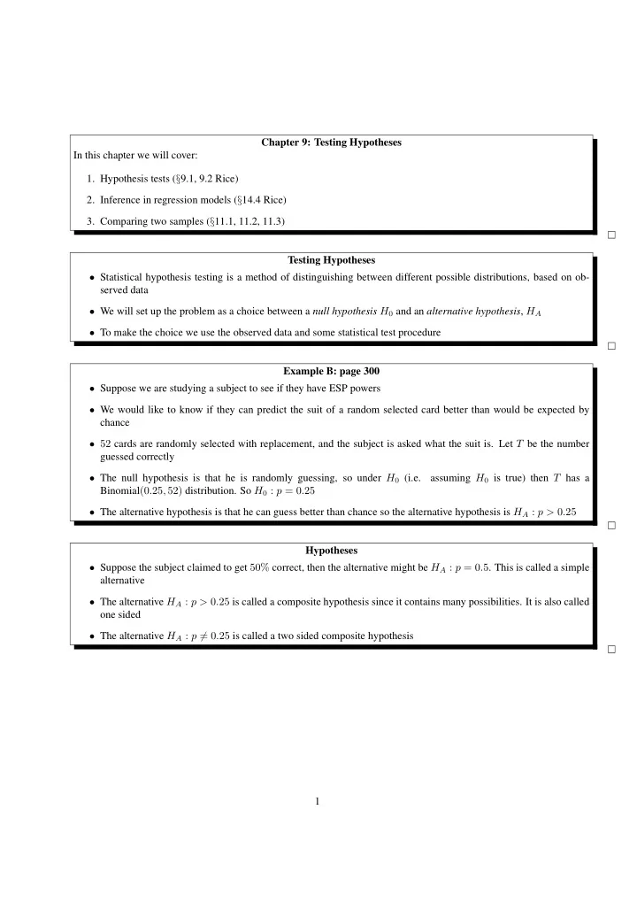
Chapter 9: Testing Hypotheses In this chapter we will cover: 1. Hypothesis tests ( § 9.1, 9.2 Rice) 2. Inference in regression models ( § 14.4 Rice) 3. Comparing two samples ( § 11.1, 11.2, 11.3) Testing Hypotheses • Statistical hypothesis testing is a method of distinguishing between different possible distributions, based on ob- served data • We will set up the problem as a choice between a null hypothesis H 0 and an alternative hypothesis , H A • To make the choice we use the observed data and some statistical test procedure Example B: page 300 • Suppose we are studying a subject to see if they have ESP powers • We would like to know if they can predict the suit of a random selected card better than would be expected by chance • 52 cards are randomly selected with replacement, and the subject is asked what the suit is. Let T be the number guessed correctly • The null hypothesis is that he is randomly guessing, so under H 0 (i.e. assuming H 0 is true) then T has a Binomial (0 . 25 , 52) distribution. So H 0 : p = 0 . 25 • The alternative hypothesis is that he can guess better than chance so the alternative hypothesis is H A : p > 0 . 25 Hypotheses • Suppose the subject claimed to get 50% correct, then the alternative might be H A : p = 0 . 5 . This is called a simple alternative • The alternative H A : p > 0 . 25 is called a composite hypothesis since it contains many possibilities. It is also called one sided • The alternative H A : p � = 0 . 25 is called a two sided composite hypothesis 1
Neyman-Pearson paradigm • We want to choose between H 0 and H A , and we make this decision based on a statistic T which is a function of the observed data X • The set of values for T for which we accept H 0 is called the acceptence region • The set of values for T for which we reject H 0 is called the rejection region • Note that we always use the choice: accept or reject H 0 . We don’t say accept H A . Errors • One possible error we might have made was to reject H 0 when it is in fact true. This is called a type I error. • The probability of type I error is called α , the significance level • The second type of possible error is to accept H 0 when it is false. This is called type II error • The probability of type II error is called β , and often 1 − β is called the power • A good test would have small α and small β Example B • We want to test H 0 : p = 0 . 25 against H A : p > 0 . 25 in the ESP example • The test statistic is T the number of correct guesses • We choose an acceptence region to be: accept H 0 if T < T 0 • What value would you choose for T 0 ? • Suppose we choose T 0 = 18 what would α and β be? 2
Example B Null distribution of T ● ● 0.12 ● Acceptence Rejection region region ● 0.10 ● Binomial(0.25, 52) probabilities ● 0.08 ● 0.06 ● ● 0.04 ● ● 0.02 ● ● ● ● ● 0.00 ● ● ● ● ● ● ● ● ● ● ● ● ● ● ● ● ● ● ● ● ● ● ● ● ● ● ● ● ● ● ● ● ● ● ● ● ● 0 10 20 30 40 50 Test statistic Example B • The size of the test defined by T 0 = 18 is the probability of rejection H 0 when H 0 is true • Thus α = P ( T ≥ 18 | p = 0 . 25) = 1 − P ( T ≤ 17 | p = 0 . 25) = 1 − F (17) = 0 . 078 where F ( x ) is the cdf for the Binomial (90 . 25 , 52) distribution • So this choice of T 0 has a small probability of committing type I error 3
Example B • To calculate β , the probability of type II error we need to calculate P (Accept H 0 | H A ) • The value of this will depend on the actual value of p in H A • Thus if p = 0 . 5 we can calculate β = P ( T < 18 | p = 0 . 5) • This can be calculated from the cdf for a Binomial (0 . 5 , 52) distribution. It equals 0 . 008 . • Since the size of β depends on the value of p a power curve, which plots 1 − β against p is a useful tool Example B: Power curve Power curve 1.0 0.8 0.6 Power 0.4 0.2 0.0 0.0 0.2 0.4 0.6 0.8 1.0 Probability Example B: Power curve • We see that the test defined by T 0 = 18 has high power for any alternative greater than 0 . 5 • It is not very powerful against p = 0 . 3 • You have to choose the acceptence region to trade of good size and good power. You can’t have both all the time. 4
Questions • If we choose T 0 = 25 would the size α increase or decrease? • What would happen to the power curve? Recommended Questions Look from § 9.12 questions 1, 2, 3, 5, 14 Regression Examples • Suppose we have a simple regression model Y i = β 0 + β 1 X i + e i which satisfies the assumptions of Chapter 14 • We have the least squares regression estimates for β 0 and β 1 . These are the same as the maximum likelihood estimates for the parameters • We can therefore ask what are confidence intervals for ˆ β 0 and ˆ β 1 ? Confidence Intervals • Just as with the example above to build the confidence intervals we need to know about the standard error of the estimates • We have from Chapter 14 that the standard errors s ˆ β i can be calculated from � n i =1 x 2 V ar (ˆ i σ 2 β 0 ) = n � n i − ( � n i =1 x i ) 2 i =1 x 2 nσ 2 V ar (ˆ β 1 ) = n � n i − ( � n i =1 x i ) 2 i =1 x 2 by the formula � V ar (ˆ β i ) s ˆ β i = n 5
Confidence Intervals • We can then use the fact that for large enough samples the distribution of ˆ β i − β i s ˆ β i has a t n − p distribution, where p is the number of terms in the regression. • The 95% confidence intervals for ˆ β i are given by � � ˆ β i , ˆ β i − t n − p (0 . 025) s ˆ β i + t n − p (0 . 025) s ˆ β i • It is of interest to see if β 1 = 0 lies inside the confidence interval Hypothesis tests • The previous analysis can also be used to test the hypthesis β 1 = 0 • The Null model is then Y i = β 0 + e i • This is asking; is there a linear relationship between the explanatory variable and the response? • Freedman makes clear that this is not testing if the explanatory variable causes the change in the response. 6
Example Democratic Congress Seats/Votes 1900−1970 80 + + + 70 + + + + + + 60 + + + + + Seat % + + + + + + + 50 + + + + + + + + + + + + 40 + + + 30 40 45 50 55 Votes % 7
Example • Here is some output from a computer package which has fitted the linear regression Estimate Std. Error beta0 -50.1821 6.9424 beta1 2.0845 0.1385 • Thus we can easily calculate the confidence intervals for β 0 is ( − 50 . 1821 − t 35 (0 . 025)6 . 9424 , − 50 . 1821 + t 35 (0 . 025)6 . 9424) = ( − 64 . 28 , − 36 . 09) and for β 1 (2 . 0845 − 2 . 03 × 0 . 1385 , 2 . 0845 + 2 . 03 × 0 . 138) = (1 . 80 , 2 . 36) • It is clear that β 1 = 0 lies a long way from the confidence interval Example: Q40 page 562 Rice • Cogswell studied a method of measuring resistence to breathing in children. He looked at two groups: asthma and cystic fibrosis patients • He wanted to investigate if there was a relationship between the height of the patient, H and the resistence R • He tried fitting a regression model R i = β 0 + β 1 H i + e i • After fitting we need to consider if β 1 = 0 is consistent with the data 8
Example: Q40 page 562 Rice Asthma patients Cystic Fibrosis + + 25 20 + 20 + + + 15 + + + resistence resistence + + 15 + + + + + + + + + + + + + + + + + + + 10 + + + + + 10 + + + + + + + + + + + + + + + + + + + + + + + + + + + 5 + + + + 90 110 130 150 90 95 100 110 height (cm) height (cm) Example: Q40 page 562 Rice • From the fit we find that for the asthma patients the fitted values are ˆ β 0 = 27 . 5157( s.e. = 6 . 63) , ˆ β 1 = − 0 . 136 , ( s.e. = 0 . 053) • The 95% confidence interval for β 1 is therefore ( − 0 . 253 , − 0 . 019) . Note that 0 does not lie inside this interval. • For the cystic fibrosis patients the fitted values are ˆ β 0 = 23 . 8( s.e. = 9 . 63) , ˆ β 1 = − 0 . 125( s.e. = 0 . 0941) • Now the 95% confidence interval for β 1 is ( − 0 . 32 , 0 . 07) . This does contain 0 so it might be that there is no relationship between height and resistence for these patients 9
Recommend
More recommend
Explore More Topics
Stay informed with curated content and fresh updates.
