Chapter 8 Forecasting Demand Qualitative Forecasting Methods Moving - PDF document

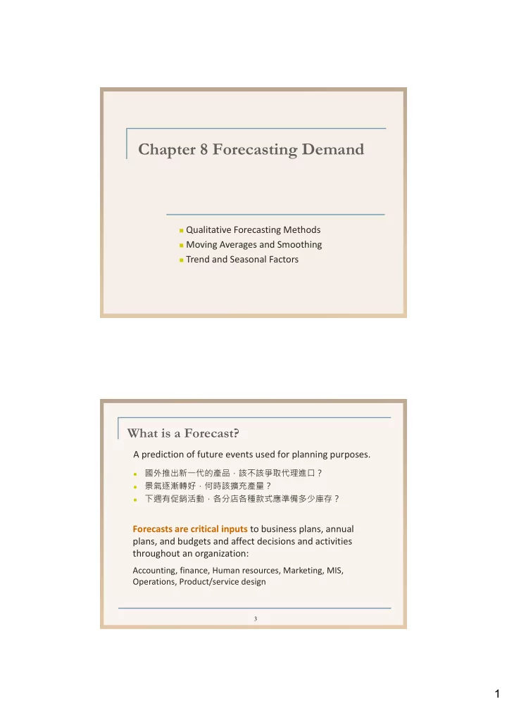
Chapter 8 Forecasting Demand  Qualitative Forecasting Methods  Moving Averages and Smoothing  Trend and Seasonal Factors What is a Forecast? A prediction of future events used for planning purposes. 國外推出新一代的產品，該不該爭取代理進口？  景氣逐漸轉好，何時該擴充產量？  下週有促銷活動，各分店各種款式應準備多少庫存？  Forecasts are critical inputs to business plans, annual plans, and budgets and affect decisions and activities throughout an organization: Accounting, finance, Human resources, Marketing, MIS, Operations, Product/service design 3 1

Demand Patterns noise trend+noise Quantity Quantity Time Time season+noise cycle Quantity Quantity Year 1 Year 2 | | | | | | | | | | | | | | | | | | 1 2 3 4 5 6 J F M A M J J A S O N D Years Months 4 Demand Management Options  The process of changing demand patterns using one or more demand options 主動影響市場需求  Complementary Products  Promotional Pricing  Revenue Management  Prescheduled Appointments supply demand  Reservations  Backlogs  Backorders and Stockouts 6 2

Key Decisions on Making Forecasts  Deciding What to Forecast  Level of aggregation: clustering several similar services or products so that forecasts are more accurate.  Choosing the Type of Forecasting Technique  Judgment methods, Causal methods, Time‐series analysis Rules of Forecasting  Forecasts are not perfect. 預測永遠是錯誤的  Forecasts for groups of items tend to be more accurate 整體預測較準確  Forecast accuracy decreases as the time horizon increases. 越久遠的預測越不準確 7 Judgment (Qualitative) Methods  Forecasts based on contextual knowledge gained through experience.  Salesforce estimates  Executive opinion  Market research Strengths  Delphi method • 可針對缺乏市場數據的新產品進行預測 • 可加入無法量化的資訊 Weaknesses • 需要良好的問卷設計與調查方式 • 意見可能偏頗、分歧、或受到不當影響 8 3

Forecast Error  It is important to measure and monitor the accuracy of forecasts. E t = D t – F t  Forecast error for a given period: F t = forecast for period t , D t = actual demand in period t n   D F t t M ean A bsolute D eviation =  t 1 n n   D F D t t t   t 1 100 % M ean A bsolute P ercentage E rror = n 9 Causal Forecasting (using Linear Regression) 估計可事先觀察的因素對於需求或銷售的影響程度 ( x 1 , …, x n ) ( y 1 , …, y n ) 可事先觀察的數值 要預測的數值 如房地產銷售 如家電銷售 假設兩者的因果關係為線性變化  Y = a + b  X 影響程度(斜率)   x y n x y i i   b i   a y b x 2  2 x n x i i 10 4

Linear Regression Regression equation: Forecast error Y = a + b  X Y Forecast of y from Dependent variable regression equation Actual Value of y Value of x used to forecast y X Independent variable 11 Example 8.2 A manager seeks to forecast the demand for door hinges and believes that the demand is related to advertising expenditures. Month Sales (thousands of units) Advertising (thousands of $) 1 264 2.5 2 116 1.3 3 165 1.4 4 101 1.0 5 209 2.0 The company will spend $1,750 next month on advertising for the product. Use causal method to develop a forecast for this product. 12 5

Example 8.2 250 – X Sales (000 units) 200 – X    1560 . 8 5 1 . 64 171 150 – X   b 109 . 229   2 14 . 9 5 ( 1 . 64 ) X 100 – X   a 8 . 135 50 – | | 0 – 1.0 2.0 Advertising ($000) Y = –8.135 + 109.229 X Forecast for next month : Y = –8.135 + 109.229(1.75) = 183.016 13 Correlation  Cause 14 6

Time Series Forecasting These methods assume that the past demand pattern will continue in the future. 過去的銷售變化型態會持續到未來 Time‐series analysis identifies underlying patterns of demand that combine to a model to forecast future demands. 15 Naïve Forecast The forecast for the next period equals the demand for the current period.  Stable time series data F(t+1) = D(t)  Seasonal variations F(t+1) = D(t+1‐n)  Data with trends F(t+1) = D(t) + (D(t) – D(t‐1)) 外插法 Works best when the horizontal, trend, or seasonal patterns are stable and random variation is small. 17 7

Horizontal Patterns: Simple Moving Averages Sum of last n demands D t + D t -1 + D t -2 + … + D t - n +1 F t +1 = = n n Example 8.3 Week Patient Arrivals 1 400 2 380 3 411 a. Compute a three‐week moving average forecast for week 4. c. If the actual number of patient arrivals in week 4 is 415, what is the forecast for week 5? 18 Large values of n should be used for demand series that are stable, and small values of n should be used for those that are susceptible to changes in the underlying average. 19 8

Horizontal Patterns: Weighted Moving Averages Assumption: 近期的數據有較高的參考價值 F t +1 = W 1 D t + W 2 D t -1 + … + W n D t - n +1 Σ W i =1 W 1 > W 2 >…> W n Example 3: Week Patient Arrivals 1 400 F t = 0.5 D t ‐1 + 0.3 D t ‐2 + 0.2 D t ‐3 2 380  F 4 = 0.50(411)+0.30(380)+0.20(400) 3 411 = 399.5 W 1 =0.5, W 2 =0.3, W 3 =0.2 20 Horizontal Patterns: Exponential Smoothing  A sophisticated weighted moving average that calculates the average of a time series by implicitly giving recent demands more weight than earlier demands 由複雜的加權平均演化而成  Requires only three items of data  The last period’s forecast  The demand for this period  A smoothing parameter, alpha ( α ), where 0 ≤ α ≤ 1.0 F t +1 = α (Demand this period) + (1– α ) (Forecast calculated last period) = α D t + (1 – α ) F t = F t + α ( D t – F t ) 21 9

Example 8.4 Week Patient Arrivals 1 400 2 380 3 411 Calculate the exponential smoothing forecast (  = 0.10) for week 4. Assume F 3 =( D 1 + D 2 )/2=390 F 4 = α D 3 + (1 – α ) F 3 = 0.10(411) + 0.90(390) = 392.1 If the actual demand for week 4 turned out to be 415, what is the forecast for week 5? F 5 = 0.10(415) + 0.90(392.1) = 394.4 22 Using Exponential Smoothing F t +1 = α D t + (1 – α ) F t Approaches to obtain an initial forecast F 1 = 前一期的銷售量 F 1 = 先前幾期的平均銷售量 F 1 =a subjective estimate smoothing constant α  Larger α values emphasize recent levels of demand and result in forecasts more responsive to changes in the underlying average.  Smaller α values treat past demand more uniformly and result in more stable forecasts. 23 10

Trend Patterns using Linear Regression A trend in a time series is a systematic increase or decrease in the average of the series over time. Indep. variable X (time)  dependent variable Y (demand) Regression 估計市場需求 (Y) 隨著時間 (X) 演進的線性關係 Y = a + b  X 該期的產品 要預測之未來 需求預測 的時期編號   趨勢(斜率) x y n x y i i     b a y b x i 2  2 x n x i i 24 Example 8.5 Arrivals at Medanalysis, Inc. Week Arrivals Week Arrivals 1 28 9 61 2 27 10 39 3 44 11 55 4 37 12 54 5 35 13 52 6 53 14 60 7 38 15 60 8 57 16 75 What is the forecasted demand for the next three periods? 25 11

Example 8.5 80   x y n x y 70 i i   b i 60 2  2 x n x 50 i i 40   a y b x 30 20 10 y =28.5+2.3456 x 0 0 5 10 15 20 Forecast for next 3 months: Y 17 = 28.5 + 2.3456(17) = 68.375 Y 18 = 28.5 + 2.3456(18) = 70.721 Y 19 = 28.5 + 2.3456(19) = 73.066 26 Seasonal Patterns: Using Seasonal Factors Seasonal patterns are regularly repeating upward or downward movements in demand measured in periods of less than one year (hours, days, weeks, months, or quarters). Additive seasonal method Add a constant to the estimate of average demand per season. Multiplicative seasonal method Seasonal factors are multiplied by an estimate of average demand 27 12

Multiplicative Seasonal Method 1. For each year, calculate the average demand for each season by dividing annual demand by the number of seasons per year. 2. For each year, divide the actual demand for each season by the average demand per season, resulting in a seasonal factor for each season. 3. Calculate the average seasonal factor for each season using the results from Step 2. 4. Calculate each season’s forecast for next year. 第 1 季 275  0.8=220 第 1 季 第 2 季 第 3 季 第 4 季 設次年的全年 第 2 季 275  1.4=385 200 350 300 150 預測 =1100 第 3 季 275  1.2=330 0.8 1.4 1.2 0.6 第 4 季 275  0.6=165 28 Example 8.6 The carpet cleaning business is seasonal, with a peak in the third quarter and a trough in the first quarter. YEAR 1 YEAR 2 YEAR 3 YEAR 4 Q1 45 70 100 100 Q2 335 370 585 725 Q3 520 590 830 1160 Q4 100 170 285 215 Total 1,000 1,200 1,800 2,200 The manager wants to forecast demand for each quarter of year 5. 29 13