Chapter 6 Orthogonality and Least Squares Section 6.1 Inner - PowerPoint PPT Presentation
Chapter 6 Orthogonality and Least Squares Section 6.1 Inner Product, Length, and Orthogonality Orientation We are now aiming at the last topic . Almost solve the equation Ax = b Problem: In the real world, data is imperfect . x u v But
Chapter 6 Orthogonality and Least Squares
Section 6.1 Inner Product, Length, and Orthogonality
Orientation We are now aiming at the last topic . ◮ Almost solve the equation Ax = b Problem: In the real world, data is imperfect . x u v But due to measurement error, the measured x is not actually in Span { u , v } . But you know, for theoretical reasons , it must lie on that plane. What do you do? The real value is probably the closest point , on the plane, to x . New terms: Orthogonal projection (‘closest point’), orthogonal vectors, angle.
The Dot Product The dot product encodes the notion of angle between two vectors. We will use it to define orthogonality (i.e. when two vectors are perpendicular) Definition The dot product of two vectors x , y in R n is x 1 y 1 x 2 y 2 def x · y = · = x 1 y 1 + x 2 y 2 + · · · + x n y n . . . . . . . x n y n This is the same as x T y . Example 1 4 4 · = = � � 2 5 1 2 3 5 3 6 6
Properties of the Dot Product Many usual arithmetic rules hold, as long as you remember you can only dot two vectors together, and that the result is a scalar . ◮ x · y = y · x ◮ ( x + y ) · z = x · z + y · z ◮ ( cx ) · y = c ( x · y ) Dotting a vector with itself is special: x 1 x 1 x 2 x 2 = x 2 1 + x 2 2 + · · · + x 2 · . . n . . . . . x n x n Hence: ◮ x · x ≥ 0 ◮ x · x = 0 if and only if x = 0. � 1 � 0 � � Important: x · y = 0 does not imply x = 0 or y = 0. For example, · = 0. 0 1
The Dot Product and Length Definition The length or norm of a vector x in R n is � x � = √ x · x = � x 2 1 + x 2 2 + · · · + x 2 n . Why is this a good definition? The Pythagorean theorem ! � � 3 4 3 2 + 4 2 = 5 � �� √ � 3 3 2 + 4 2 = 5 � � � = � � 4 4 � √ 3 Fact If x is a vector and c is a scalar , then � cx � = | c | · � x � . � � 6 �� � � 3 �� � � � � � = � 2 � = � � � � 8 4 �
The Dot Product and Distance The following is just the length of the vector from x to y . Definition The distance between two points x , y in R n is dist( x , y ) = � y − x � . Example Let x = (1 , 2) and y = (4 , 4). Then dist( x , y ) = y y − x x 0
Unit Vectors Definition A unit vector is a vector v with length � v � = 1. Example The unit coordinate vectors are unit vectors: � � 1 � � � 1 2 + 0 2 + 0 2 = 1 � � � e 1 � = 0 = � � � � 0 � � Definition Let x be a nonzero vector in R n . The unit vector in the direction of x is the x vector � x � . Is this really a unit vector? � � 1 x � � � = � x �� x � = 1 . scalar � � � x � �
Unit Vectors Example Example � 3 � What is the unit vector in the direction of x = ? 4
Orthogonality Definition Two vectors x , y are orthogonal or perpendicular if x · y = 0. Notation: Write it as x ⊥ y . Why is this a good definition? The Pythagorean theorem / law of cosines! y � x − y � � y � x � x � ⇒ � x − y � 2 = � x � 2 + � y � 2 (Pythagorean Theorem) Fact: x ⊥ y ⇐
Orthogonality Example 1 Problem: Find all vectors orthogonal to v = 1 . − 1 We have to find all vectors x such that x · v = 0. This means solving the equation x 1 1 · = x 1 + x 2 − x 3 . 0 = x · v = x 2 1 x 3 − 1
Orthogonality Example 1 1 and w = Problem: Find all vectors orthogonal to both v = 1 1 . − 1 1 Now we have to solve the system of two homogeneous equations x 1 1 · = x 1 + x 2 − x 3 0 = x · v = x 2 1 x 3 − 1 x 1 1 · = x 1 + x 2 + x 3 . 0 = x · w = x 2 1 1 x 3
Orthogonality General procedure Problem: Find all vectors orthogonal to v 1 , v 2 , . . . , v m in R n . This is the same as finding all vectors x such that 0 = v T 1 x = v T 2 x = · · · = v T m x . — v T 1 — v 1 · x Putting the row vectors v T 1 , v T 2 , . . . , v T m — v T 2 — v 2 · x into a matrix, this is the same as finding . . x = = 0 . . . . . all x such that — v T v m · x m — The key observation — v T 1 — The set of all vectors orthogonal to some vec- tors v 1 , v 2 , . . . , v m in R n is the null space of — v T 2 — . . . . the m × n matrix: — v T m —
Orthogonal Complements Definition Let W be a subspace of R n . Its orthogonal complement is W ⊥ = v in R n | v · w = 0 for all w in W � � read “ W perp”. W ⊥ is orthogonal complement A T is transpose Pictures: The orthogonal complement of a line in R 2 is the W W ⊥ perpendicular line. W W ⊥ The orthogonal complement of a line in R 3 is the perpendicular plane. W ⊥ W The orthogonal complement of a plane in R 3 is the perpendicular line.
Poll
Orthogonal Complements Basic properties Facts: Let W be a subspace of R n . 1. W ⊥ is also a subspace of R n 2. ( W ⊥ ) ⊥ = W 3. dim W + dim W ⊥ = n 4. If W = Span { v 1 , v 2 , . . . , v m } , then W ⊥ = all vectors orthogonal to each v 1 , v 2 , . . . , v m x in R n | x · v i = 0 for all i = 1 , 2 , . . . , m � � = — v T 1 — — v T 2 — . = Nul . . . — v T m — Property 4 — v T 1 — — v T 2 — Span { v 1 , v 2 , . . . , v m } ⊥ = Nul . . . — v T m —
Orthogonal Complements Row space, column space, null space Definition The row space of an m × n matrix A is the span of the rows of A . It is denoted Row A . Equivalently, it is the column span of A T : Row A = Col A T . It is a subspace of R n . We showed before that if A has rows v T 1 , v T 2 , . . . , v T m , then Span { v 1 , v 2 , . . . , v m } ⊥ = Nul A . Hence we have shown: (Row A ) ⊥ = Nul A .
Extra: Reference sheet Orthogonal Complements of Most of the Subspaces We’ve Seen For any vectors v 1 , v 2 , . . . , v m : — v T 1 — — v T 2 — (Span { v 1 , v 2 , . . . , v m } ) ⊥ = Nul . . . — v T m — For any matrix A : Row A = Col A T thus (Row A ) ⊥ = Nul A Row A = (Nul A ) ⊥ (Col A ) ⊥ = Nul A T Col A = (Nul A T ) ⊥
Extra: Practice proving a set is subspace and some facts
Recommend
More recommend
Explore More Topics
Stay informed with curated content and fresh updates.
