Chapter 22: Elementary Graph Algorithms. Definitions : 1. G = ( V, E - PDF document

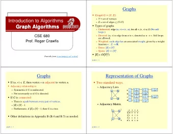
Chapter 22: Elementary Graph Algorithms. Definitions : 1. G = ( V, E ), where V is a set of points and E is a set of edges connecting point-pairs from V . 2. We use V synonymously with | V | and E with | E | when the context is clear. 3. Adjacency list representation: randomly addressable vector V , with attributes as needed in an application, e.g. v.color, v.cnt. One attribute is v.adj, which holds a pointer to a linked list of edges leaving vertex v. 4. Adjacency list structure can be scanned in Θ( V + E ) time. 1

5. Adjacency matrix representation: V × V matrix M with M ij holding infor- mation about the edge, if any, between vertices i and j . Typically, vertices are represented as 1 , 2 , 3 , . . . , and we need a parallel structure to hold vertex attributes. Matrix cells can hold edge attributes. 6. Adjacency matrix structure can be scanned in Θ( V 2 ) time. 7. E = o ( V 2 ) implies the list structure is more efficient; E = Θ( V 2 ) implies the matrix structure is equally efficient. 2

Algorithm for calculating the out-degree of each vertex, given an adjacency list representation. Get-out-degree(V) { for u ∈ V loop { V + 1 u.out-degree = 0 V � V for v ∈ u.adj loop i =1 ( n i + 1), where n i is the edge count of u � V u.out-degree = u.out-degree + 1 i =1 n i } } Since E = � V i =1 n i , we have T = 3 V + 2 E + 1 = Θ( V + E ). For a graph g , code will look more like... Vertex[ ] u = g. vertices; // returns vertex vector Edge e = null; for (int i = 0; i < u. length; i + +) { u [ i ] . out-degree = 0; e = u. adj; while ( e ! = null) { u. out-degree = u. out-degree + 1; e = e. next; } } 3

Algorithm for calculating the in-degree of each vertex, given an adjacency list representation. Get-in-degree(V) { for u ∈ V loop V + 1 u.in-degree = 0 V for u ∈ V loop V + 1 � V for v ∈ u.adj loop i =1 ( n i + 1), where n i is the edge count of u � V v.in-degree = v.in-degree + 1 i =1 n i } Since E = � V i =1 n i , we have T = 4 V + 2 E + 2 = Θ( V + E ). 4

Algorithm for calculating the transpose graph, given an adjacency list representa- tion. Get-transpose(V) { for u ∈ V loop V + 1 u.trans-adj = null V for u ∈ V loop V + 1 � V for v ∈ u.adj loop i =1 ( n i + 1), where n i is the edge count of u � V add u to v.trans-adj i =1 n i } Since E = � V i =1 n i , we have T = 4 V + 2 E + 2 = Θ( V + E ). 5

Algorithm for eliminating self-loops and multiple edges, given an adjacency list representation. Get-reduction(V) { for u ∈ V loop { V + 1 u. reduced-adj = null; V u. mark = null; V } for u ∈ V loop V + 1 � V for v ∈ u. adj loop { i =1 ( n i + 1), where n i is the edge count of u � V if ( v � = u ) and ( v. mark � = u ) { i =1 n i 0 to 2 � V add v to u. reduced-adj; i =1 n i v. mark = u ; } } } Observations: 1. Failure of the if-test implies the two following lines are not executed. Success implies they are both executed. Hence the count for the pair is zero in the best-case and 2 � V i =1 n i in the worst-case. 2. Since � V i =1 n i = E , we have 5 V + 2 E + 2 ≤ T ≤ 5 V + 4 E + 2, implying T = Θ( V + E ). 3. When the first vertex starts processing as u , all v .mark values are null. As pro- cessing continues for u these v .mark values remain either null or u , depending on whether edge ( u, v ) has been seen. When the second vertex starts process- ing as u , all v .mark values are either null or the previous vertex. During the processing of this second u , the mark values may be null, or the first vertex, or the second vertex. And so forth. Hence we never need to reset the mark attribute for subsequent values u values in the outer loop. 6

Algorithm for calculating G 2 , given an adjacency list representation. If G = ( V, E ), G 2 = ( V, E 2 ), where (u, v) ∈ E 2 if and only if (a) (u, v) ∈ E or (b) there exist a vertex w with (u, w) ∈ E and (w, v) ∈ E . (First step in constructing the transitive closure) Get-transitive( V ) { for u ∈ V loop { V + 1 u. trans-adj = null; V � V for v ∈ u. adj loop { i =1 ( n i + 1) = E + V � V add v to u. trans-adj; i =1 n i = E for w ∈ v. adj loop E + EV (max) add w to u. trans-adj; EV (max) } } } run Get-reduction on G , using the trans-adj edges, to remove duplicate edges } Observations: 1. Third-level loop is initiated for each ( u, v ) edge. The max-count occurs if destination vertex v is connected to all of V . 2. Last operation to remove duplicate edges is linear: Θ( V + E ). 3. Complexity, worst case, = 3 V + 2 EV + 3 E + 1 + Θ( V + E ) = 2 EV + Θ( V + E ) T � Θ( V 3 ) , E = Θ( V 2 ) = Θ( V 2 ) , E = Θ( V ) . 7

Compare adjacency matrix solution. [ a ij ] is the given adjacency matrix; [ b ij ] is matrix of transitive augmentation. Assume graph has n vertices. Get-transitive( a, b ) { for i = 1 to n loop V + 1 for j = 1 to n loop V ( V + 1) if a ij = 1 b ij = 1; else { b ij = 0; for k = 1 to n loop if a ik a kj == 1 { b ij = 1; exit k -loop; } } } The first if-statement executes V 2 times. In a shortest execution, the statement will always succeed, adding 2 V 2 to the 2 V 2 + 2 V + 1 noted in the code. In a longest execution, the statement will always fail, the subsequent if-statement always succeeds, and the exit will not be taken, adding V 2 [2 + ( V + 1) + 3 V ] to the 2 V 2 + 2 V + 1 noted in the code. T ( n ) ≥ 2 V 2 + 2 V + 1 + 2 V 2 = 4 V 2 + 2 V + 1 T ( n ) ≤ 2 V 2 + 2 V + 1 + 2 V 2 + V 3 + V 2 + 3 V 3 = 4 V 3 + 5 V 2 + 2 V + 1 T ( n ) = Ω( V 2 ) T ( n ) = O ( V 3 ) , which is comparable to the adjacency list approach. 8

Breadth-first Search (BFS) while Q � = φ loop { BFS( G, s ) // G = ( V, E ) , s ∈ V { u = Q. dequeue(); for v ∈ V \{ s } loop { for v ∈ u. adj loop { v .color = white; if v. color = white { v.d = ∞ ; v. color = gray; v.π = null v.d = u.d + 1; } v.π = u ; s .color = gray; Q. enqueue( v ); s.d = 0; } s.π = null; } Q = φ ; u. color = black; Q. enqueue( s ); } } Observations: 1. Setup: Θ( V ) While-loop: Each v ∈ V is enqueued at most once and assigned gray just prior to enqueue operation. Also no vertex ever reverts to white, which implies O ( V ) while-loop iterations. Each iteration processes a disjoint set of edge links. Consequently, the while-loop activity is O ( V + E ). BFS is then O ( V + E ). 2. Cannot guarantee Ω( V + E ) as the component containing s might remain small as the graph size expands toward infinity, which would cause (instruction count)/( V + E ) → 0 as size increases. 9

Definition : δ ( s, v ) is the shortest number of links in a path from s to v , if such a path exists. Otherwise, δ ( s, v ) = ∞ . Lemma 22.1 (triangle inequality) : ( u, v ) ∈ E ⇒ δ ( s, v ) ≤ δ ( s, u ) + 1. Proof: If δ ( s, u ) = ∞ , desired result is certainly true. Otherwise, any path from s to u , including the shortest one of length δ ( s, u ), followed by edge ( u, v ), is a competitor for δ ( s, v ), which implies the desired inequality. 10

We assume an adjacency list representa- tion for the undirected graph to the left. The numbers specify the order in which edges appears on the various edge lists The vertex queue evolves as follows. Each vertex is represented a column vector. The top position records the vertex; the middle position records the .d value; the final position records the .π value ( φ means null). s s w r s w r t x s w r t x v s w r t x v u 0 ⇒ 0 1 1 ⇒ 0 1 1 2 2 ⇒ 0 1 1 2 2 2 ⇒ 0 1 1 2 2 2 3 φ φ s s φ s s w w φ s s w w r φ s s w w r t s w r t x v u y s w r t x v u y ⇒ 0 1 1 2 2 2 3 3 ⇒ 0 1 1 2 2 2 3 3 φ s s w w r t x φ s s w w r t x s w r t x v u y s w r t x v u y ⇒ 0 1 1 2 2 2 3 3 ⇒ 0 1 1 2 2 2 3 3 φ s s w w r t x φ s s w w r t x The queue content is the segment between the two vertical lines. left of the first vertical line (black) ⇒ removed from the queue between the lines (gray) ⇒ evolving as the last removed item adds vertices from its adjacency list Process assigns a .π value to each vertex, except s , that identifies the previous vertex leading to its discovery. We use these ancestor marks to evolve the following G π tree. 11

s w r t x v u y 0 1 1 2 2 2 3 3 φ s s w w r t x 12

Lemma 22.2 : G = ( V, E ), directed or undirected. On termination of BFS( G, s ), v.d ≥ δ ( s, v ) for all v ∈ V . Proof: (Via induction on the number of enqueue operations) We note that v.d is changed at most once for each v ∈ V . For nodes that do not pass through the queue, v.d = ∞ , its initial value, at all times during the algorithm execution. Hence, for these nodes v.d = ∞ ≥ δ ( v, s ) holds at the conclusion of the algorithm. For all other vertices, we note that its d attribute is changed just before it is enqueued. As a base case, the first such enqueue operation places s in the queue. At that point, we have s.d = 0 = δ ( s, s ). At this time, s.d = 0 = δ ( s, s ), and δ ( s, v ) = ∞ for all other vertices v . Hence the inequality holds after the first enqueue operation. Consider now a later enqueue of node v . The v.d value is set just before it enters the queue. Specifically, v.d = u.d + 1 for a neighbor u that has already passed through the queue. By induction, we can assume u.d ≥ δ ( u, s ). So, v.d = u.d + 1 ≥ δ ( s, u ) + 1 ≥ δ ( s, v ) , the last equality following because ( u, v ) ∈ E and the triangle inequality applies. 13