
Chapter 2 State Space Models General format : (valid for any - PDF document
Chapter 2 State Space Models General format : (valid for any nonlinear causal system) CT : x = f ( x, u ) , DT : x k +1 = f ( x k , u k ) , y = h ( x, u ) . y k = h ( x k , u k ) . where x = the state of the system, n 1-vector u
✬ ✩ Chapter 2 State Space Models General format : (valid for any nonlinear causal system) CT : ˙ x = f ( x, u ) , DT : x k +1 = f ( x k , u k ) , y = h ( x, u ) . y k = h ( x k , u k ) . where x = the state of the system, n × 1-vector u = the input of the system, m × 1-vector y = the output of the system, p × 1-vector f = state equation vector function h = output equation vector function n = number of states ⇒ n -th order system m = number of inputs p = number of outputs Single-Input Single-Output system (SISO) : m = p = 1, Multi-Input Multi-Output system (MIMO) : m, p > 1, Multi-Input Single-Output system (MISO) : m > 1 , p = 1, Single-Input Multi-Output system (SIMO) : m = 1 , p > 1. ✫ ✪ CACSD pag. 34 ESAT–SCD–SISTA
✬ ✩ Linear Time Invariant (LTI) systems (only valid for linear causal systems) Continuous-time system: x = Ax + Bu ˙ y = Cx + Du x ˙ x � u y B C A D Discrete-time system: x k +1 = Ax k + Bu k y k = Cx k + Du k x k +1 x k u k y k z − 1 B C A D A: n × n system matrix B: n × m input matrix C: p × n output matrix D: p × m direct transmission matrix ✫ ✪ CACSD pag. 35 ESAT–SCD–SISTA
✬ ✩ An example of linear state space modeling: Example: Tape drive control - state space modeling Process description: p 1 p 3 p 2 D D β r β r K K J J θ 2 θ 1 i 1 i 2 + + e 1 e 2 K t K t − − The drive motor on each end of the tape is independently controllable by voltage resources e 1 and e 2 . The tape is modeled as a linear spring with a small amount of viscous damping near to the static equilibrium with tape tension 6N. The variables are defined as deviations from this equi- librium point. ✫ ✪ CACSD pag. 36 ESAT–SCD–SISTA
✬ ✩ The equations of motion of the system are: J dω 1 capstan 1: dt = Tr − βω 1 + K t i 1 , speed of x 1 : p 1 = rω 1 , ˙ Ldi 1 motor 1: dt = − Ri 1 − K e ω 1 + e 1 , J dω 2 capstan 2: dt = − Tr − βω + K t i 2 , speed of x 1 : p 2 = rω 2 , ˙ Ldi 2 motor 2: dt = − Ri 2 − K e ω 2 + e 2 , T = K 2 ( p 2 − p 1 ) + D Tension of tape: 2 ( ˙ p 2 − ˙ p 1 ) , p 3 = p 1 + p 2 Position of the head: . 2 ✫ ✪ CACSD pag. 37 ESAT–SCD–SISTA
✬ ✩ Description of variables and constants: D = damping in the tape-stretch motion = 20 N/m · sec, e 1 , 2 = applied voltage, V, i 1 , 2 = current into the capstan motor, J = inertia of the wheel and the motor = 4 × 10 − 5 kg · m 2 , β = capstan rotational friction, 400kg · m 2 /sec, K = spring constant of the tape, 4 × 10 4 N/m, K e = electrical constant of the motors = 0.03V · sec, K t = torque constant of the motors = 0.03N · m/A, L = armature inductance = 10 − 3 H, R = armature resistance = 1Ω, r = radius of the take-up wheels, 0.02m, T = tape tension at the read/write head, N , p 1 , 2 , 3 = tape position at capstan 1,2 and the head, p 1 , 2 , 3 = tape velocity at capstan 1,2 and the head, ˙ θ 1 , 2 = angular displacement of capstan 1,2, ω 1 , 2 = speed of drive wheels = ˙ θ 1 , 2 . ✫ ✪ CACSD pag. 38 ESAT–SCD–SISTA
✬ ✩ With a time scaling factor of 10 3 and a position scaling fac- tor 10 − 5 for numerical reasons, the state equations become: x = Ax + Bu, ˙ y = Cx + Du, where p 1 0 2 0 0 0 0 ω 1 − 0 . 1 − 0 . 35 0 . 1 0 . 1 0 . 75 0 p 2 0 0 0 2 0 0 x = , A = ω 2 0 . 1 0 . 1 − 0 . 1 − 0 . 35 0 0 . 75 i 1 0 − 0 . 03 0 0 − 1 0 i 2 0 0 0 − 0 . 03 0 − 1 0 0 0 0 � � 0 0 0 . 5 0 0 . 5 0 0 0 B = , C = , 0 0 − 0 . 2 − 0 . 2 0 . 2 0 . 2 0 0 1 0 0 1 � � � � � � 0 0 p 3 e 1 D = , y = , u = . 0 0 T e 2 ✫ ✪ CACSD pag. 39 ESAT–SCD–SISTA
✬ ✩ State-space model, transfer matrix and impulse response Continuous-time system: Laplace � state-space x = Ax + Bu ˙ G ( s ) = Y ( s ) x (0)=0 U ( s ) = D + C ( sI − A ) − 1 B − → equations y = Cx + Du � �� � transfer matrix in practice : D = 0 ⇓ ∞ Laplace � G ( t ) = Ce At B CA i − 1 Bs − i ← → G ( s ) = � �� � i =1 impulse response matrix � �� � transfer matrix Discrete-time system: z − transf � state-space x k +1 = Ax k + Bu k G ( z ) = Y ( z ) x 0 =0 U ( z ) = D + C ( zI − A ) − 1 B ← → equations y k = Cx k + Du k � �� � transfer matrix ⇓ � ∞ D : k = 0 z − transf � CA i − 1 Bz − i + D G ( k ) = ← → G ( z ) = CA k − 1 B : k ≥ 1 i =1 � �� � � �� � impulse response matrix transfer matrix In case of a SISO system, G ( t ) or G ( k ) is the impulse response. For MIMO G ( t ), G ( k ) are matrices containing the m × p impulse responses (one for every input-output pair). ✫ ✪ CACSD pag. 40 ESAT–SCD–SISTA
✬ ✩ Linearization of a nonlinear system about an equilibrium point Consider a general nonlinear system in continuous time : dx dt = f ( x, u ) y = h ( x, u ) For small deviations about an equilibrium point ( x e , u e , y e ) for which f ( x e , u e ) = 0 y e = h ( x e , u e ) we define x = x e + ∆ x, u = u e + ∆ u, y = y e + ∆ y, and obtain dx dt = d ∆ x = f ( x, u ) = f ( x e + ∆ x, u e + ∆ u ) dt and y e + ∆ y = h ( x, u ) = h ( x e + ∆ x, u e + ∆ u ) . ✫ ✪ CACSD pag. 41 ESAT–SCD–SISTA
✬ ✩ By first order approximation we obtain a linear state space model from ∆ u to ∆ y : d ∆ x = f ( x e + ∆ x, u e + ∆ u ) dt ⇓ f ( x e , u e ) = 0 � � d ∆ x = ∂f ∆ x + ∂f (1) � � ∆ u � � dt ∂x ∂u � � x e ,u e x e ,u e � �� � � �� � n × n n × m ⇓ ⇓ A B and y e + ∆ y = h ( x e + ∆ x, u e + ∆ u ) ⇓ y e = h ( x e , u e ) � � = ∂h ∆ x + ∂h (1) � � ∆ y ∆ u � � ∂x ∂u � � x e ,u e x e ,u e � �� � � �� � p × n p × m ⇓ ⇓ C D Conclusion : use a linear approximation about equilibrium. ✫ ✪ CACSD pag. 42 ESAT–SCD–SISTA
✬ ✩ Example : Consider a decalcification plant which is used to reduce the concentration of calcium hydroxide in water by forming a calcium carbonate precipitate. The following equations hold (simplified model) : • chemical reaction : Ca(OH) 2 + CO 2 → CaCO 3 + H 2 O • reaction speed : r = c [Ca(OH) 2 ][CO 2 ] • rate of change of concentration : d [Ca(OH) 2 ] = k V − r dt V d [CO 2 ] = u V − r dt V k and u are the inflow rates in moles/second of calcium hydroxide and carbon dioxide respectively. V is the tank volume in liters. Let the inflow rate of carbon dioxide be the input and the concentration of calcium hydroxide be the output. ✫ ✪ CACSD pag. 43 ESAT–SCD–SISTA
✬ ✩ A nonlinear state space model for this reactor is : d [Ca(OH) 2 ] = k V − c V [Ca(OH) 2 ][CO 2 ] dt d [CO 2 ] = u V − c V [Ca(OH) 2 ][CO 2 ] dt y = [Ca(OH) 2 ] The state variables are x 1 = [Ca(OH) 2 ] and x 2 = [CO 2 ]. In equilibrium we have : V − c k V [Ca(OH) 2 ] eq [CO 2 ] eq = k V − c V X 1 X 2 = 0 u eq V − c V [Ca(OH) 2 ] eq [CO 2 ] eq = U V − c V X 1 X 2 = 0 Y = [Ca(OH) 2 ] eq = X 1 For small deviations about the equilibrium : d ∆ x 1 = − c V X 2 ∆ x 1 − c V X 1 ∆ x 2 dt d ∆ x 2 = − c V X 2 ∆ x 1 − c V X 1 ∆ x 2 + 1 V ∆ u dt ∆ y = ∆ x 1 so, � � � � − cX 2 − cX 1 0 � � V V A = , B = , C = , D = 0 1 0 − cX 2 − cX 1 1 V V V ✫ ✪ CACSD pag. 44 ESAT–SCD–SISTA
✬ ✩ If k = 0 . 1 mole U = 0 . 1 mole l 2 sec , c = 0 . 5 sec · mole, sec , X 1 = 0 . 25 mole , X 2 = 0 . 8 mole , V = 5 l l l then − 0 . 08 − 0 . 025 0 � � A B = − 0 . 08 − 0 . 025 0 . 2 C D 1 0 0 The corresponding transfer function is ∆ y ( s ) − 0 . 005 ∆ u ( s ) = s 2 + 0 . 105 s and its bode plot Bode Diagrams 50 0 Phase (deg); Magnitude (dB) −50 −250 −300 −350 −400 −3 −2 −1 0 10 10 10 10 Frequency (rad/sec) ✫ ✪ CACSD pag. 45 ESAT–SCD–SISTA
✬ ✩ One can also obtain a linear state space model for this chemical plant from linear system identification. For small deviations about the equilibrium point the dy- namics can be described fairly well by a linear ( A, B, C, D )- model. Hence, a small white noise disturbance ∆ u was generated and was added to the equilibrium value U . We applied this signal to the input of a nonlinear model of the chemical reactor (Simulink model for instance), i.e. u ( t ) = U + ∆ u . The following input-output set was obtained : u(t) 0.104 0.102 0.1 0.098 0.096 0 100 200 300 400 500 600 700 800 900 1000 time (s) y(t) 0.2505 0.25 0.2495 0.249 0 100 200 300 400 500 600 700 800 900 1000 time (s) ✫ ✪ CACSD pag. 46 ESAT–SCD–SISTA
Recommend


More recommend
Explore More Topics
Stay informed with curated content and fresh updates.