Chapter 15: Dynamic Programming. Rod-cutting problem. Given: rod of - PDF document
Chapter 15: Dynamic Programming. Rod-cutting problem. Given: rod of integer length n inches a table of retail values (dollars for rods of integer lengths) Problem: cut the rod to maximize retail value For example: length i 1 2 3 4 5 6 7
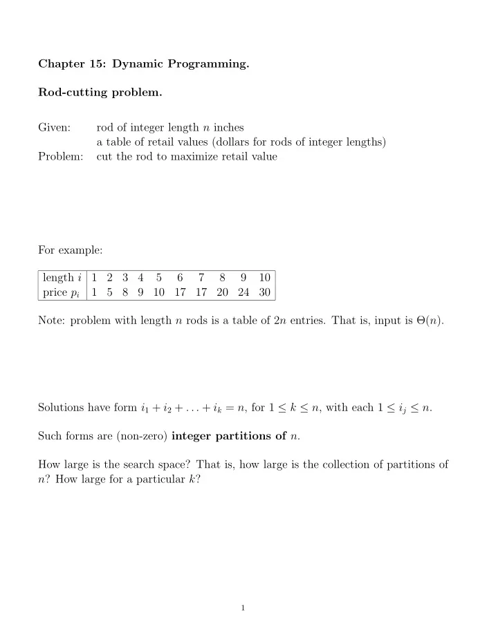
Chapter 15: Dynamic Programming. Rod-cutting problem. Given: rod of integer length n inches a table of retail values (dollars for rods of integer lengths) Problem: cut the rod to maximize retail value For example: length i 1 2 3 4 5 6 7 8 9 10 price p i 1 5 8 9 10 17 17 20 24 30 Note: problem with length n rods is a table of 2 n entries. That is, input is Θ( n ). Solutions have form i 1 + i 2 + . . . + i k = n , for 1 ≤ k ≤ n , with each 1 ≤ i j ≤ n . Such forms are (non-zero) integer partitions of n . How large is the search space? That is, how large is the collection of partitions of n ? How large for a particular k ? 1
The star-bar visualization . For n = 4 , k = 3 and allowing elements of size | | * * * * 004 zero, we obtain the | * | * * * 013 | * * | * * 022 � n + ( k − 1) � � 4 + 3 − 1 � � 6 � = = = 15 | * * * | * 031 k − 1 2 2 | * * * * | 040 configurations to the left. * | | * * * 103 If we reserve 3 of the 4 stars to ensure that each * | * | * * 112 element is at least one: * | * * | * 121 | | * 001 ⇒ 112 * | * * * | 130 | * | 010 ⇒ 121 * * | | * * 202 * | | 100 ⇒ 211 * * | * | * 211 � n − k + ( k − 1) � � n − 1 � * * | * * | 220 = k − 1 k − 1 * * * | | * 301 * * * | * | 310 � 4 − 1 � � 3 � = = = 3 . * * * * | | 400 3 − 1 2 If N n is the number of non-zero partitions of n , then n n − 1 � n − 1 � � n − 1 � = 2 n − 1 = 1 � � 2 · 2 n , N n = = k − 1 k k =1 k =0 an exponential search space. 2
A recursive solution. Let r n = maximum retail value that can be obtained from a rod of length n r 0 = 0 r n = 1 ≤ i ≤ n ( p i + r n − i ) . max Note optimal substructure . RecursiveCutRod( p, n ) { if n = 0 return 0; q = −∞ ; for i = 1 to n q = max ( q, p [ i ] + RecursiveCutRod( p, n − i )); return q ; } What is the instruction count growth rate as n → ∞ ? 3
For a simple lower bound, let T ( n ) count only the recursive calls — no work done therein. T (0) = 0 n n − 1 � � T ( n ) = n + T ( n − i ) = n + T ( i ) i =1 i =0 0 � T (1) = 1 + T ( i ) = 1 + T (0) = 1 i =0 1 � T (2) = 2 + T ( i ) = 2 + T (0) + T (1) = 2 + 1 + 0 = 3 i =0 2 � T (3) = 3 + T ( i ) = 3 + 3 + 1 + 0 = 7 i =0 3 � T (4) = 4 + T ( i ) = 4 + 7 + 3 + 1 + 0 = 15 i =0 Conjecture: T ( n ) = 2 n − 1. Verify: n − 1 n − 1 n − 1 2 i = 2 n − 1 (2 i − 1) = n − n + 2 − 1 = 2 n − 1 . � � � n + T ( i ) = n + i =0 i =0 i =0 So, T ( n ), which undercounts the instruction count of RecursiveCutRod, is Ω(2 n ), which is as bad as a brute-force search of the entire solution space. 4
Why? The same recursive subproblem occurs many times under different activation records. Better approach: keep an array of subproblem solutions. History: In the early days of computation, “programming” meant filling in a grid (array) Bellman (1940-50s) used “dynamic” to conceal mathematics at Rand from an unenlightened Secretary of State (Wilson) (Wikipedia) BottomUpCutRod( p, n ) { n + 1 r [0 . . . n ] = 0; n + 1 for j = 1 to n { n q = −∞ ; � n j =1 ( j + 1) for i = 1 to j � n j =1 j q = max ( q, p [ i ] + r [ j − i ]); n r [ j ] = q ; } } T ( n ) = 5 n + 2 + 2 � n j =1 j = 5 n + 2 + n ( n + 1) = Θ( n 2 ). 5
If T ′ ( n ) counts the number of references, T ′ ( n ) = � n j =1 j = n ( n +1) = Θ( n 2 ), imply- 2 ing T ( n ) = Θ( n 2 ) because each reference involves Θ(1) work. 6
Definitions. 1. Memoization : Record intermediate results for later use. 2. Bottom-up : compute all required sub-problems before using them. 3. Top-down : compute overall solution via a recursive call that computes only the necessary sub-problems ( lazy evaluation ). MemoizedCutRod( p, n ) { r [0 . . . n ] = 0; return Aux( p, n, r ); } Aux( p, n, r ) { if r [ n ] > 0 return r [ n ]; if n = 0 q = 0; else { q = −∞ ; for i = 1 to n q = max ( q, p [ i ] + Aux( p, n − i, r )); } r [ n ] = q ; return q ; } Count Aux calls in sketch ( n = 5): 5 + 4 + 3 + 2 + 1 = 15. In general, n j = n ( n + 1) � = Θ( n 2 ) . T ( n ) = 2 j =1 7
Reconstituting the cuts. ExtendedBottomUpCutRod( p, n ) { ( n + 1) r [0 . . . n ] = 0; ( n + 1) for j = 1 to n { ( n ) q = −∞ ; �� n � j =1 ( j + 1) for i = 1 to j { �� n � j =1 j x = p [ i ] + r [ j − i ]; �� n � j =1 (3 j ) if q < x { q = x ; s [ j ] = i ; ← parallel structure records decision } } ( n ) r [ j ] = q ; } (1) return r, s ; } n j = 5 n + 3 + 5 n ( n + 1) � = Θ( n 2 ) . T ( n ) = 5 n + 3 + 5 2 j =1 i 0 1 2 3 4 5 6 7 8 9 10 p [ i ] 0 1 5 8 9 10 17 17 20 24 30 r [ i ] 0 1 5 8 10 13 17 18 22 25 30 s [ i ] 0 1 2 3 2 2 6 1 2 3 10 e.g. 5 → 2 → 3 → 0 In general, n → s [ n ] → s [ n − s [ n ]] → s [ n − s [ n ] − s [ n − s [ n ]]] → . . . → 0. 8
PrintCutRodSolution( p, n ) { ( r, s ) = ExtendedBottomUpCutRod( p, n ) { while n > 0 { print( s [ n ]); n = n − s [ n ]; } } Variation that foreshadows greedy approach (Chapter 16). Let the value density be the retail dollars per inch, ρ i = p i /i . A greedy approach cuts the segment with the highest density and continues to so cut the remainder. i 0 1 2 3 4 5 6 7 8 9 10 p [ i ] 0 1 5 8 9 10 17 17 20 24 30 r [ i ] 0 1 5 8 10 13 17 18 22 25 30 s [ i ] 0 1 2 3 2 2 6 1 2 3 10 ρ [ i ] 1.00 2.50 2.67 2.25 2.00 2.83 2.43 2.50 2.67 3.00 Note for n = 4, greedy approach finds max { 1 . 00 , 2 . 50 , 2 . 67 , 2 . 25 } = 2 . 67 and chooses decomposition 4 = 3 + 1 yielding $9.00. DP approach gives 4 = 2 + 2 for a yield of $10.00. 9
Identifying characteristics of a dynamic programming opportunity. 1. Exponential search space 2. Optimal substructure property: An optimal solution contains optimal solutions of independent subproblems. 3. Recursive solution repeats subproblem solutions. 4. Dynamic Programming stores subproblem solutions for re-use. DP requires the appropriate storage structure and a scan-order that ensures each subprob- lem is available when needed. 5. Optimal objective function value typically in the last cell computed in the storage structure. 6. The corresponding search space object can be constructed from a parallel stor- age structure that records the optimal decisions. 10
Example regarding independent subproblems. Let G = ( V, E ) be an unweighted graph. For u, v ∈ V , define � ∞ , no paths from u to v δ ( u, v ) = min { # of links in p : p is a path from u to v } , ∃ p : u � v. If p : ( u = v 0 , v 1 , . . . , v k = v ) is a shortest path from u to v , then p ′ : ( v i , v i +1 , . . . , v j ) is a shortest path from v i to v j for 0 ≤ i < j ≤ k . This optimal substructure property follows from a cut-and-paste proof. However, suppose δ ( u, v ) = # of links in the longest simple path from u to v. δ ( q, t ) = 2 via q → r → t . However q → r is not the longest simple path from q to r , as its path length (1) is beaten by q → s → t → r with a length of 3. Also, it is not possible to assemble longest paths of subproblems to obtain a longest path for an overall problem. For example, q → s → t → r and r → q → s → t are the longest simple paths from q to r and from r to t respectively. But, q → s → t → r → q → s → t is not even a simple path. Independent subproblems means no sharing of resources (edges in this example). 11
Matrix Chain Multiplication. Consider matrices A 1 (10 × 100) , A 2 (100 × 5) , A 3 (5 × 50). A 1 A 2 A 3 via ( A 1 A 2 ) A 3 ⇒ (10)(100)(5) + (10)(5)(50) = 7500 multiplications. A 1 A 2 A 3 via A 1 ( A 2 A 3 ) ⇒ (100)(5)(50) + (10)(100)(50) = 75000 multiplications. We seek an optimal grouping (parenthesization) of A 1 A 2 . . . A n to multiply with the smallest number of multiplications. A 1 : ( p 0 × p 1 ) A 2 : ( p 1 × p 2 ) ⇒ ( p 0 × p n ) . . . A n : ( p n − 1 × p n ) How many groupings? Search space size = ? Let P ( n ) be the number of parenthesis configurations for n multiplication-compatible matrices. P (1) = P (2) = 1. A 1 A 2 A 3 ⇒ A 1 ( A 2 A 3 ) or ( A 1 A 2 ) A 3 . So, P(3) = 2. In general, the outermost grouping is A 1 . . . A k and A k +1 . . . A n for 1 ≤ k ≤ n − 1. n − 1 � P ( n ) = P ( k ) P ( n − k ) k =1 b k = P ( k + 1) n n n − 1 � � � b n = P ( n + 1) = P ( k ) P ( n − k + 1) = b k − 1 b n − k = b k b n − k − 1 k =1 k =1 k =0 ∞ � b n x n B ( x ) = n =0 B 2 ( x ) = ( b 0 + b 1 x + b 2 x 2 + . . . )( b 0 + b 1 x + b 2 x 2 + . . . ) = b 2 0 + x ( b 0 b 1 + b 1 b 0 ) + x 2 ( b 0 b 2 + b 1 b 1 + b 2 b 0 ) + x 3 ( b 0 b 3 + b 1 b 2 + b 2 b 1 + b 3 b 0 ) 12
B 2 ( x ) = c 0 + c 1 x + c 2 x 2 + . . . + c n x n + . . . n � c n = b k b n − k k =0 n − 1 � c n − 1 = b k b n − k − 1 = b n k =0 B 2 ( x ) = b 1 + b 2 x + b 3 x 2 + . . . xB 2 ( x ) = b 1 x + b 2 x 2 + b 3 x 3 + . . . = B ( x ) − b 0 b 0 = P (1) = 1 xB 2 ( x ) = B ( x ) − 1 xB 2 ( x ) − B ( x ) + 1 = 0 B ( x ) = 1 ± √ 1 − 4 x 2 x Want lim x → 0 B ( x ) = b 0 = 1. We have 1 + √ 1 − 4 x lim = ∞ 2 x x → 0 + 1 + √ 1 − 4 x lim = −∞ 2 x x → 0 − 1 − √ 1 − 4 x − (1 / 2)(1 − 4 x ) − 1 / 2 ( − 4) 1 lim = lim = lim (1 − 4 x ) 1 / 2 = 1 . 2 x 2 x → 0 x → 0 x → 0 We conclude B ( x ) = 1 − √ 1 − 4 x . 2 x Expand √ 1 − 4 x as a power series about x = 0. 13
Recommend
More recommend
Explore More Topics
Stay informed with curated content and fresh updates.
