Centrality Measures and Link Analysis Gonzalo Mateos Dept. of ECE - - PowerPoint PPT Presentation

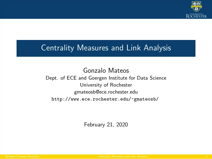
Centrality Measures and Link Analysis

Gonzalo Mateos

• Dept. of ECE and Goergen Institute for Data Science

University of Rochester gmateosb@ece.rochester.edu http://www.ece.rochester.edu/~gmateosb/

February 21, 2020

Network Science Analytics Centrality Measures and Link Analysis 1

Centrality measures

Centrality measures Case study: Stability of centrality measures in weighted graphs Centrality, link analysis and web search A primer on Markov chains PageRank as a random walk PageRank algorithm leveraging Markov chain structure

Network Science Analytics Centrality Measures and Link Analysis 2

Quantifying vertex importance

◮ In network analysis many questions relate to vertex importance

Example

◮ Q1: Which actors in a social network hold the ‘reins of power’? ◮ Q2: How authoritative is a WWW page considered by peers? ◮ Q3: The ‘knock-out’ of which genes is likely to be lethal? ◮ Q4: How critical to the daily commute is a subway station? ◮ Measures of vertex centrality quantify such notions of importance

⇒ Degrees are simplest centrality measures. Let’s study others

Network Science Analytics Centrality Measures and Link Analysis 3

Closeness centrality

◮ Rationale: ‘central’ means a vertex is ‘close’ to many other vertices ◮ Def: Distance d(u, v) between vertices u and v is the length of the

shortest u − v path. Oftentimes referred to as geodesic distance

◮ Closeness centrality of vertex v is given by

cCl(v) = 1

• u∈V d(u, v)

◮ Interpret v ∗ = arg maxv cCl(v) as the most approachable node in G

Network Science Analytics Centrality Measures and Link Analysis 4

Normalization, computation and limitations

◮ To compare with other centrality measures, often normalize to [0, 1]

cCl(v) = Nv − 1

• u∈V d(u, v)

◮ Computation: need all pairwise shortest path distances in G

⇒ Dijkstra’s algorithm in O(N2

v log Nv + NvNe) time ◮ Limitation 1: sensitivity, values tend to span a small dynamic range

⇒ Hard to discriminate between central and less central nodes

◮ Limitation 2: assumes connectivity, if not cCl(v) = 0 for all v ∈ V

⇒ Compute centrality indices in different components

Network Science Analytics Centrality Measures and Link Analysis 5

Betweenness centrality

◮ Rationale: ‘central’ node is (in the path) ‘between’ many vertex pairs ◮ Betweenness centrality of vertex v is given by

cBe(v) =

• s=t=v∈V

σ(s, t|v) σ(s, t)

◮ σ(s, t) is the total number of s − t shortest paths ◮ σ(s, t|v) is the number of s − t shortest paths through v ∈ V

◮ Interpret v ∗ = arg maxv cBe(v) as the controller of information flow

Network Science Analytics Centrality Measures and Link Analysis 6

Computational considerations

◮ Notice that a s − t shortest path goes through v if and only if

d(s, t) = d(s, v) + d(v, t)

◮ Betweenness centralities can be naively computed for all v ∈ V by:

Step 1: Use Dijkstra to tabulate d(s, t) and σ(s, t) for all s, t Step 2: Use the tables to identify σ(s, t|v) for all v Step 3: Sum the fractions to obtain cBe(v) for all v (O(N3

v ) time)

◮ Cubic complexity can be prohibitive for large networks ◮ O(NvNe)-time algorithm for unweighted graphs in:

• U. Brandes, “A faster algorithm for betweenness centrality,” Journal
• f Mathematical Sociology, vol. 25, no. 2, pp. 163-177, 2001

Network Science Analytics Centrality Measures and Link Analysis 7

Eigenvector centrality

◮ Rationale: ‘central’ vertex if ‘in-neighbors’ are themselves important

⇒ Compare with ‘importance-agnostic’ degree centrality

◮ Eigenvector centrality of vertex v is implicitly defined as

cEi(v) = α

• (u,v)∈E

cEi(u)

1

2 3 4 5 6

◮ No one points to 1 ◮ Only 1 points to 2 ◮ Only 2 points to 3, but 2

more important than 1

◮ 4 as high as 5 with less links ◮ Links to 5 have lower rank ◮ Same for 6

Network Science Analytics Centrality Measures and Link Analysis 8

Eigenvalue problem

◮ Recall the adjacency matrix A and

cEi(v) = α

• (u,v)∈E

cEi(u)

◮ Vector cEi = [cEi(1), . . . , cEi(Nv)]⊤ solves the eigenvalue problem

AcEi = α−1cEi ⇒ Typically α−1 chosen as largest eigenvalue of A [Bonacich’87]

◮ If G is undirected and connected, by Perron’s Theorem then

⇒ The largest eigenvalue of A is positive and simple ⇒ All the entries in the dominant eigenvector cEi are positive

◮ Can compute cEi and α−1 via O(N2 v ) complexity power iterations

cEi(k + 1) = AcEi(k) AcEi(k), k = 0, 1, . . .

Network Science Analytics Centrality Measures and Link Analysis 9

Example: Comparing centrality measures

◮ Q: Which vertices are more central? A: It depends on the context ◮ Each measure identifies a different vertex as most central

⇒ None is ‘wrong’, they target different notions of importance

Network Science Analytics Centrality Measures and Link Analysis 10

Example: Comparing centrality measures

◮ Q: Which vertices are more central? A: It depends on the context

Closeness Betweenness Eigenvector

◮ Small green vertices are arguably more peripheral

⇒ Less clear how the yellow, dark blue and red vertices compare

Network Science Analytics Centrality Measures and Link Analysis 11

Case study

Centrality measures Case study: Stability of centrality measures in weighted graphs Centrality, link analysis and web search A primer on Markov chains PageRank as a random walk PageRank algorithm leveraging Markov chain structure

Network Science Analytics Centrality Measures and Link Analysis 12

Centrality measures robustness

◮ Robustness to noise in network data is of practical importance ◮ Approaches have been mostly empirical

⇒ Find average response in random graphs when perturbed ⇒ Not generalizable and does not provide explanations

◮ Characterize behavior in noisy real graphs

⇒ Degree and closeness are more reliable than betweenness

◮ Q: What is really going on?

⇒ Framework to study formally the stability of centrality measures

◮ S. Segarra and A. Ribeiro, “Stability and continuity of centrality

measures in weighted graphs,” IEEE Trans. Signal Process., 2015

Network Science Analytics Centrality Measures and Link Analysis 13

Definitions for weighted digraphs

◮ Weighted and directed graphs G(V , E, W )

⇒ Set V of Nv vertices ⇒ Set E ⊆ V × V of edges ⇒ Map W : E → R++ of weights in each edge

a b c 5 4 2 3 ◮ Path P(u, v) is an ordered sequence of nodes from u to v ◮ When weights represent dissimilarities

⇒ Path length is the sum of the dissimilarities encountered

◮ Shortest path length sG(u, v) from u to v

sG(u, v) := min

P(u,v) ℓ−1

• i=0

W (ui, ui+1)

Network Science Analytics Centrality Measures and Link Analysis 14

Stability of centrality measures

◮ Space of graphs G(V ,E) with (V , E) as vertex and edge set ◮ Define the metric d(V ,E)(G, H) : G(V ,E) × G(V ,E) → R+

d(V ,E)(G, H) :=

• e∈E

|WG(e) − WH(e)|

◮ Def: A centrality measure c(·) is stable if for any vertex v ∈ V in any

two graphs G, H ∈ G(V ,E), then

• cG(v) − cH(v)
• ≤ KG d(V ,E)(G, H)

◮ KG is a constant depending on G only ◮ Stability is related to Lipschitz continuity in G(V ,E) ◮ Independent of the definition of d(V ,E) (equivalence of norms)

◮ Node importance should be robust to small perturbations in the graph

Network Science Analytics Centrality Measures and Link Analysis 15

Degree centrality

◮ Sum of the weights of incoming arcs

cDe(v) :=

• u|(u,v)∈E

W (u, v)

◮ Applied to graphs where the weights in W represent similarities ◮ High cDe(v) ⇒ v similar to its large number of neighbors

Proposition 1 For any vertex v ∈ V in any two graphs G, H ∈ G(V ,E), we have that |cG

De(v) − cH De(v)| ≤ d(V ,E)(G, H)

i.e., degree centrality cDe is a stable measure

◮ Can show closeness and eigenvector centralities are also stable

Network Science Analytics Centrality Measures and Link Analysis 16

Betweenness centrality

◮ Look at the shortest paths for every two nodes distinct from v

⇒ Sum the proportion that contains node v cBe(v) :=

• s=v=t∈V

σ(s, t|v) σ(s, t)

◮ σ(s, t) is the total number of s − t shortest paths ◮ σ(s, t|v) is the number of those paths going through v

Proposition 2 The betweenness centrality measure cBe is not stable

Network Science Analytics Centrality Measures and Link Analysis 17

Instability of betweenness centrality

◮ Compare the value of cBe(v) in graphs G and H

G v 1 1 1 1 1 1 1 1 cG

Be(v) = 9

H v 1 + ǫ 1 + ǫ 1 1 1 1 1 1 cH

Be(v) = 0

⇒ Centrality value cH

Be(v) = 0 remains unchanged for any ǫ > 0 ◮ For small values of ǫ, graphs G and H become arbitrarily similar

9 = |cG

Be(v) − cH Be(v)| ≤ KG d(V ,E)(G, H) → 0

⇒ Inequality is not true for any constant KG

Network Science Analytics Centrality Measures and Link Analysis 18

Stable betweenness centrality

◮ Define G v =(V v, E v, W v), V v=V \{v}, E v=E|V v×V v , W v=W |E v

⇒ G v obtained by deleting from G node v and edges connected to v

◮ Stable betweenness centrality cSBe(v)

cSBe(v) :=

• s=v=t∈V

sG v (s, t) − sG(s, t) ⇒ Captures impact of deleting v on the shortest paths

◮ If v is (not) in the s − t shortest path, sG v (s, t) − sG(s, t) > (=)0

⇒ Same notion as (traditional) betweenness centrality cBe Proposition 3 For any vertex v ∈ V in any two graphs G, H ∈ G(V ,E), then |cG

SBe(v) − cH SBe(v)| ≤ 2N2 v d(V ,E)(G, H)

i.e., stable betweenness centrality cSBe is a stable measure

Network Science Analytics Centrality Measures and Link Analysis 19

Centrality ranking variation in random graphs

◮ Gn,p graphs with p = 10/n and weights U(0.5, 1.5)

⇒ Vary n from 10 to 200 ⇒ Perturb multiplying weights with random numbers U(0.99, 1.01)

◮ Compare centrality rankings in the original and perturbed graphs

20 40 60 80 100 120 140 160 180 200 2 4 6 8 10

Network Size Mean maximum change in ranking

CD CC CB CE CSB 20 40 60 80 100 120 140 160 180 200 0.2 0.4 0.6 0.8 1 1.2 1.4

Network Size Mean average change in ranking

CD CC CB CE CSB

◮ Betweenness centrality presents larger maximum and average changes

Network Science Analytics Centrality Measures and Link Analysis 20

Centrality ranking variation in random graphs

◮ Compute probability of observing a ranking change ≥ 5

⇒ Plot the histogram giving rise to the empirical probabilities

20 40 60 80 100 120 140 160 180 200 0.2 0.4 0.6 0.8 1

Network Size Probability max change greater than 5

CD CC CB CE CSB 1 2 3 4 5 6 7 8 9 10 11 12 13 14 15 16 17 18 19 20 10 20 30 40 50 60

Maximum change in ranking Frequency

CD CC CB CE CSB

◮ For cBe some node varies its ranking by 5 positions with high probability ◮ Long tail in histogram is evidence of instability

⇒ Minor perturbation generates change of 19 positions

Network Science Analytics Centrality Measures and Link Analysis 21

Centrality ranking variation in an airport graph

◮ Real-world graph based on the air traffic between popular U.S. airports

⇒ Nodes are Nv = 25 popular airports ⇒ Edge weights are the number of yearly passengers between them

5 10 15 20 25 30 35 40 45 50 0.1 0.2 0.3 0.4 0.5 0.6 0.7 0.8 0.9

Perturbation Size (1000 x δ) Probability max change greater than 1

CD CC CB CE CSB 1 2 3 4 5 6 10 20 30 40 50 60 70 80 90

Maximum change in ranking Frequency

CD CC CB CE CSB

◮ Betweenness centrality still presents the largest variations

Network Science Analytics Centrality Measures and Link Analysis 22

Centrality, link analysis and web search

Centrality measures Case study: Stability of centrality measures in weighted graphs Centrality, link analysis and web search A primer on Markov chains PageRank as a random walk PageRank algorithm leveraging Markov chain structure

Network Science Analytics Centrality Measures and Link Analysis 23

The problem of ranking websites

◮ Search engines rank pages by looking at the Web itself

⇒ Enough information intrinsic to the Web and its structure

◮ Information retrieval is a historically difficult problem

⇒ Keywords vs complex information needs (synonymy, polysemy)

◮ Beyond explosion in scale, unique issues arised with the Web

◮ Diversity of authoring styles, people issuing queries ◮ Dynamic and constantly changing content ◮ Paradigm: from scarcity to abundance

◮ Finding and indexing documents that are relevant is ‘easy’ ◮ Q: Which few of these should the engine recommend?

⇒ Key is understanding Web structure, i.e., link analysis

Network Science Analytics Centrality Measures and Link Analysis 24

Voting by in-links

Ex: Suppose we issue the query ‘newspapers’

◮ First, use text-only information retrieval to identify relevant pages ◮ Idea: Links suggest implicit endorsements of other relevant pages

◮ Count in-links to assess the authority of a page on ‘newspapers’ Network Science Analytics Centrality Measures and Link Analysis 25

A list-finding technique

◮ Query also returns pages that compile lists of relevant resources

◮ These hubs voted for many highly endorsed (authoritative) pages

◮ Idea: Good lists have a better sense of where the good results are

◮ Page’s hub value is the sum of votes received by its linked pages Network Science Analytics Centrality Measures and Link Analysis 26

Repeated improvement

◮ Reasonable to weight more the votes of pages scoring well as lists

⇒ Recompute votes summing linking page values as lists

◮ Q: Why stop here? Use also improved votes to refine the list scores

⇒ Principle of repeated improvement

Network Science Analytics Centrality Measures and Link Analysis 27

Hubs and authorities

◮ Relevant pages fall in two categories: hubs and authorities ◮ Authorities are pages with useful, relevant content

◮ Newspaper home pages ◮ Course home pages ◮ Auto manufacturer home pages

◮ Hubs are ‘expert’ lists pointing to multiple authorities

◮ List of newspapers ◮ Course bulletin ◮ List of US auto manufacturers

◮ Rules: Authorities and hubs have a mutual reinforcement relationship

⇒ A good hub links to multiple good authorities ⇒ A good authority is linked from multiple good hubs

Network Science Analytics Centrality Measures and Link Analysis 28

Hubs and authorities ranking algorithm

◮ Hyperlink-Induced Topic Search (HITS) algorithm [Kleinberg’98] ◮ Each page v ∈ V has a hub score hv and authority score av

⇒ Network-wide vectors h = [h1, . . . , hNv ]⊤, a = [a1, . . . , aNv ]⊤ Authority update rule: av(k) =

• (u,v)∈E

hu(k − 1), for all v ∈ V ⇔ a(k) = A⊤h(k − 1) Hub update rule: hv(k) =

• (v,u)∈E

au(k), for all v ∈ V ⇔ h(k) = Aa(k)

◮ Initialize h(0) = 1/√Nv, normalize a(k) and h(k) each iteration

Network Science Analytics Centrality Measures and Link Analysis 29

Limiting values

◮ Define the hub and authority rankings as

a := lim

k→∞ a(k),

h := lim

k→∞ h(k) ◮ From the HITS update rules one finds for k = 0, 1, . . .

a(k + 1) = A⊤Aa(k) A⊤Aa(k), h(k + 1) = AA⊤h(k) AA⊤h(k)

◮ Power iterations converge to dominant eigenvectors of A⊤A and AA⊤

A⊤Aa = α−1

a a,

AA⊤h = α−1

h h

⇒ Hub and authority ranks are eigenvector centrality measures

Network Science Analytics Centrality Measures and Link Analysis 30

Link analysis beyond the web

Ex: link analysis of citations among US Supreme Court opinions

◮ Rise and fall of authority of key Fifth Amendment cases [Fowler-Jeon’08]

Network Science Analytics Centrality Measures and Link Analysis 31

PageRank

◮ Node rankings to measure website relevance, social influence ◮ Key idea: in-links as votes, but ‘not all links are created equal’

⇒ How many links point to a node (outgoing links irrelevant) ⇒ How important are the links that point to a node

◮ PageRank key to Google’s original ranking algorithm [Page-Brin’98] ◮ Inuition 1: fluid that percolates through the network

⇒ Eventually accumulates at most relevant Web pages

◮ Inuition 2: random web surfer (more soon)

⇒ In the long-run, relevant Web pages visited more often

◮ PageRank and HITS success was quite different after 1998

Network Science Analytics Centrality Measures and Link Analysis 32

Basic PageRank update rule

◮ Each page v ∈ V has PageRank rv, let r = [r1, . . . , rNv ]⊤

⇒ Define P := (Dout)−1A, where Dout is the out-degree matrix PageRank update rule: rv(k) =

• (u,v)∈E

ru(k − 1) dout

u

, for all v ∈ V ⇔ r(k) = PTr(k − 1)

◮ Split current PageRank evenly among outgoing links and pass it on

⇒ New PageRank is the total fluid collected in the incoming links ⇒ Initialize r(0) = 1/Nv. Flow conserved, no normalization needed

◮ Problem: ‘Spider traps’

◮ Accumulate all PageRank ◮ Only when not strongly connected Network Science Analytics Centrality Measures and Link Analysis 33

Scaled PageRank update rule

◮ Apply the basic PageRank rule and scale the result by s ∈ (0, 1)

Split the leftover (1 − s) evenly among all nodes (evaporation-rain) Scaled PageRank update rule: rv(k) = s ×

• (u,v)∈E

ru(k − 1) dout

u

+ 1 − s Nv , for all v ∈ V

◮ Can view as basic update r(k) = ¯

PTr(k − 1) with ¯ P := sP + (1 − s)11⊤ Nv ⇒ Scaling factor s typically chosen between 0.8 and 0.9 ⇒ Power iteration converges to the dominant eigenvector of ¯ PT

Network Science Analytics Centrality Measures and Link Analysis 34

A primer on Markov chains

Centrality measures Case study: Stability of centrality measures in weighted graphs Centrality, link analysis and web search A primer on Markov chains PageRank as a random walk PageRank algorithm leveraging Markov chain structure

Network Science Analytics Centrality Measures and Link Analysis 35

Markov chains

◮ Consider discrete-time index n = 0, 1, 2, . . . ◮ Time-dependent random state Xn takes values on a countable set

◮ In general denote states as i = 0, 1, 2, . . ., i.e., here the state space is N ◮ If Xn = i we say “the process is in state i at time n”

◮ Random process is XN, its history up to n is Xn = [Xn, Xn−1, . . . , X0]T ◮ Def: process XN is a Markov chain (MC) if for all n ≥ 1, i, j, x ∈ Nn

P

• Xn+1 = j
• Xn = i, Xn−1 = x
• = P
• Xn+1 = j
• Xn = i
• = Pij

◮ Future depends only on current state Xn (memoryless, Markov property)

⇒ Future conditionally independent of the past, given the present

Network Science Analytics Centrality Measures and Link Analysis 36

Matrix representation

◮ Group the Pij in a transition probability “matrix” P

P =         P00 P01 P02 . . . P0j . . . P10 P11 P12 . . . P1j . . . . . . . . . . . . . . . . . . . . . Pi0 Pi1 Pi2 . . . Pij . . . . . . . . . . . . . . . . . . ...         ⇒ Not really a matrix if number of states is infinite

◮ Row-wise sums should be equal to one, i.e., ∞ j=0 Pij = 1 for all i

Network Science Analytics Centrality Measures and Link Analysis 37

Graph representation

◮ A graph representation or state transition diagram is also used

i i +1 i −1 . . . . . . Pi,i Pi,i+1 Pi,i−1 Pi+1,i+1 Pi+1,i Pi+1,i+2 Pi−1,i−1 Pi−1,i Pi−1,i−2 Pi+2,i+1 Pi−2,i−1

◮ Useful when number of states is infinite, skip arrows if Pij = 0 ◮ Again, sum of per-state outgoing arrow weights should be one

Network Science Analytics Centrality Measures and Link Analysis 38

Example: Bipolar mood

◮ I can be happy (Xn = 0) or sad (Xn = 1)

⇒ My mood tomorrow is only affected by my mood today

◮ Model as Markov chain with transition probabilities

P =

• 0.8

0.2 0.3 0.7

• H

S 0.8 0.2 0.7 0.3

◮ Inertia ⇒ happy or sad today, likely to stay happy or sad tomorrow ◮ But when sad, a little less likely so (P00 > P11)

Network Science Analytics Centrality Measures and Link Analysis 39

Example: Random (drunkard’s) walk

◮ Step to the right w.p. p, to the left w.p. 1 − p

⇒ Not that drunk to stay on the same place

i i +1 i −1 . . . . . . p 1 − p 1 − p p p 1 − p 1 − p p

◮ States are 0, ±1, ±2, . . . (state space is Z), infinite number of states ◮ Transition probabilities are

Pi,i+1 = p, Pi,i−1 = 1 − p

◮ Pij = 0 for all other transitions

Network Science Analytics Centrality Measures and Link Analysis 40

Multiple-step transition probabilities

◮ Q: What can be said about multiple transitions? ◮ Probabilities of Xm+n given Xm ⇒ n-step transition probabilities

Pn

ij = P

• Xm+n = j
• Xm = i
• ⇒ Define the matrix P(n) with elements Pn

ij

Theorem The matrix of n-step transition probabilities P(n) is given by the n-th power of the transition probability matrix P, i.e., P(n) = Pn Henceforth we write Pn

Network Science Analytics Centrality Measures and Link Analysis 41

Unconditional probabilities

◮ All probabilities so far are conditional, i.e., Pn ij = P

• Xn = j
• X0 = i
• ⇒ May want unconditional probabilities pj(n) = P (Xn = j)

◮ Requires specification of initial conditions pi(0) = P (X0 = i) ◮ Using law of total probability and definitions of Pn ij and pj(n)

pj(n) = P (Xn = j) =

∞

• i=0

P

• Xn = j
• X0 = i
• P (X0 = i)

=

∞

• i=0

Pn

ij pi(0) ◮ In matrix form (define vector p(n) = [p1(n), p2(n), . . .]T)

p(n) = (Pn)T p(0)

Network Science Analytics Centrality Measures and Link Analysis 42

Limiting distributions

◮ MCs have one-step memory. Eventually they forget initial state ◮ Q: What can we say about probabilities for large n?

πj := lim

n→∞ P

• Xn = j
• X0 = i
• = lim

n→∞ Pn ij

⇒ Assumed that limit is independent of initial state X0 = i

◮ We’ve seen that this problem is related to the matrix power Pn

P = 0.8 0.2 0.3 0.7

• ,

P7 = 0.6031 0.3969 0.5953 0.4047

• P2 =

0.7 0.3 0.45 0.55

• ,

P30 = 0.6000 0.4000 0.6000 0.4000

• ◮ Matrix product converges ⇒ probs. independent of time (large n)

◮ All rows are equal ⇒ probs. independent of initial condition

Network Science Analytics Centrality Measures and Link Analysis 43

Limit distribution of ergodic Markov chains

Theorem For an ergodic (i.e. irreducible, aperiodic, and positive recurrent) MC, limn→∞ Pn

ij exists and is independent of the initial state i, i.e.,

πj = lim

n→∞ Pn ij

Furthermore, steady-state probabilities πj ≥ 0 are the unique nonnegative solution of the system of linear equations πj =

∞

• i=0

πiPij,

∞

• j=0

πj = 1

◮ Limit probs. independent of initial condition exist for ergodic MC

⇒ Simple algebraic equations can be solved to find πj

Network Science Analytics Centrality Measures and Link Analysis 44

Markov chains meet eigenvalue problems

◮ Define vector steady-state distribution π := [π0, π1, . . . , πJ]T ◮ Limit distribution is unique solution of

π = PTπ, πT1 = 1

◮ Eigenvector π associated with eigenvalue 1 of PT

◮ Eigenvectors are defined up to a scaling factor ◮ Normalize to sum 1

◮ All other eigenvalues of PT have modulus smaller than 1 ◮ Computing π as eigenvector is computationally efficient

Network Science Analytics Centrality Measures and Link Analysis 45

Ergodicity

◮ Def: Fraction of time T (n) i

spent in i-th state by time n is T (n)

i

:= 1 n

n

• m=1

I {Xm = i}

◮ Compute expected value of T (n) i

E

• T (n)

i

• = 1

n

n

• m=1

E [I {Xm = i}] = 1 n

n

• m=1

P (Xm = i)

◮ As n → ∞, probabilities P (Xm = i) → πi (ergodic MC). Then

lim

n→∞ E

• T (n)

i

• = lim

n→∞

1 n

n

• m=1

P (Xm = i) = πi

◮ For ergodic MCs same is true without expected value ⇒ Ergodicity

lim

n→∞ T (n) i

= lim

n→∞

1 n

n

• m=1

I {Xm = i} = πi, a.s.

Network Science Analytics Centrality Measures and Link Analysis 46

Example: Ergodic Markov chain

◮ Consider an ergodic Markov chain with transition probability matrix

P :=   0.3 0.7 0.1 0.5 0.4 0.1 0.2 0.7  

Visits to states, nT (n)

i

Ergodic averages, T (n)

i

5 10 15 20 25 30 35 40 5 10 15 20 25 time number of visits State 1 State 2 State 3 10 20 30 40 50 60 70 80 90 100 0.1 0.2 0.3 0.4 0.5 0.6 0.7 0.8 time ergodic averages State 1 State 2 State 3

◮ Ergodic averages slowly converge to π = [0.09, 0.29, 0.61]T

Network Science Analytics Centrality Measures and Link Analysis 47

PageRank: Random walk formulation

Centrality measures Case study: Stability of centrality measures in weighted graphs Centrality, link analysis and web search A primer on Markov chains PageRank as a random walk PageRank algorithm leveraging Markov chain structure

Network Science Analytics Centrality Measures and Link Analysis 48

Preliminary definitions

◮ Graph G = (V , E) ⇒ vertices V = {1, 2, . . . , J} and edges E

1 2 3 4 5 6

◮ Outgoing neighborhood of i is the set of nodes j to which i points

n(i) := {j : (i, j) ∈ E}

◮ Incoming neighborhood of i is the set of nodes that point to i:

n−1(i) := {j : (j, i) ∈ E}

◮ Strongly connected G ⇒ directed path joining any pair of nodes

Network Science Analytics Centrality Measures and Link Analysis 49

Definition of rank

◮ Agent A chooses node i, e.g., web page, at random for initial visit ◮ Next visit randomly chosen between links in the neighborhood n(i)

⇒ All neighbors chosen with equal probability

◮ If reach a dead end because node i has no neighbors

⇒ Chose next visit at random equiprobably among all nodes

◮ Redefine graph G = (V , E) adding edges from dead ends to all nodes

⇒ Restrict attention to connected (modified) graphs

1 2 3 4 5 6

◮ Rank of node i is the average number of visits of agent A to i

Network Science Analytics Centrality Measures and Link Analysis 50

Equiprobable random walk

◮ Formally, let An be the node visited at time n ◮ Define transition probability Pij from node i into node j

Pij := P

• An+1 = j
• An = i
• ◮ Next visit equiprobable among i’s Ni := |n(i)| neighbors

Pij = 1 |n(i)| = 1 Ni , for all j ∈ n(i)

1 2 3 4 5 6 to 1 to 2 to 3 to 4 to 5 1/2 1/2 1/2 1/2 1/2 1/2 1/2 1/2 1

1/5 1/5 1/5 1/5 1/5 ◮ Still have a graph ◮ But also a MC ◮ Red (not blue) circles

Network Science Analytics Centrality Measures and Link Analysis 51

Formal definition of rank

◮ Def: Rank ri of i-th node is the time average of number of visits

ri := lim

n→∞

1 n

n

• m=1

I {Am = i} ⇒ Define vector of ranks r := [r1, r2, . . . , rJ]T

◮ Rank ri can be approximated by average rni at time n

rni := 1 n

n

• m=1

I {Am = i} ⇒ Since lim

n→∞ rni = ri , it holds rni ≈ ri for n sufficiently large

⇒ Define vector of approximate ranks rn := [rn1, rn2, . . . , rnJ]T

◮ If modified graph is connected, rank independent of initial visit

Network Science Analytics Centrality Measures and Link Analysis 52

Ranking algorithm

Output : Vector r(i) with ranking of node i Input : Scalar n indicating maximum number of iterations Input : Vector N(i) containing number of neighbors of i Input : Matrix N(i, j) containing indices j of neighbors of i m = 1; r=zeros(J,1); % Initialize time and ranks A0 = random(’unid’,J); % Draw first visit uniformly at random while m < n do jump = random(’unid’,N(Am−1)); % Neighbor uniformly at random Am = N(Am−1, jump); % Jump to selected neighbor r(Am) = r(Am) + 1; % Update ranking for Am m = m + 1; end r = r/n; % Normalize by number of iterations n

Network Science Analytics Centrality Measures and Link Analysis 53

Social graph example

◮ Asked probability students about homework collaboration ◮ Created (crude) graph of the social network of students in the class

⇒ Used ranking algorithm to understand connectedness Ex: I want to know how well students are coping with the class ⇒ Best to ask people with higher connectivity ranking

◮ 2009 data from “UPenn’s ECE440”

Network Science Analytics Centrality Measures and Link Analysis 54

Ranked class graph

Aarti Kochhar

Ranga Ramachandran Saksham Karwal

Aditya Kaji Alexandra Malikova Pia Ramchandani

Amanda Smith

Amanda Zwarenstein

Jane Kim

Katie Joo Lisa Zheng Michael Harker Rebecca Gittler Lindsey Eatough Ankit Aggarwal Priya Takiar Anthony Dutcher Ciara Kennedy Carolina Lee Daniela Savoia Robert Feigenberg Ceren Dumaz Charles Jeon Chris Setian Eric Lamb Pallavi Yerramilli Ella Kim Jacci Jeffries Harish Venkatesan Ivan Levcovitz Jesse Beyroutey Jihyoung Ahn Madhur Agarwal Owen Tian Xiang-Li Lim Paul Deren Varun Balan Thomas Cassel Shahid Bosan Sugyan Lohiaa

Network Science Analytics Centrality Measures and Link Analysis 55

Convergence metrics

◮ Recall r is vector of ranks and rn of rank iterates ◮ By definition

lim

n→∞ rn = r . How fast rn converges to r (r given)? ◮ Can measure by ℓ2 distance between r and rn

ζn := r − rn2 =

• J
• i=1

(rni − ri)2 1/2

◮ If interest is only on highest ranked nodes, e.g., a web search

⇒ Denote r (i) as the index of the i-th highest ranked node ⇒ Let r (i)

n

be the index of the i-th highest ranked node at time n

◮ First element wrongly ranked at time n

ξn := arg min

i {r (i) = r (i) n }

Network Science Analytics Centrality Measures and Link Analysis 56

Evaluation of convergence metrics

Distance

1000 2000 3000 4000 5000 6000 7000 8000 9000 10000 10

−2

10

−1

10 10

1

time (n) correctly ranked nodes

First element wrongly ranked

1000 2000 3000 4000 5000 6000 7000 8000 9000 10000 2 4 6 8 10 12 14 time (n) correctly ranked nodes

◮ Distance close to 10−2 in

≈ 5 × 103 iterations

◮ Bad: Two highest ranks

in ≈ 4 × 103 iterations

◮ Awful: Six best ranks in

≈ 8 × 103 iterations

◮ (Very) slow convergence

Network Science Analytics Centrality Measures and Link Analysis 57

When does this algorithm converge?

◮ Cannot confidently claim convergence until 105 iterations

⇒ Beyond particular case, slow convergence inherent to algorithm

0.2 0.4 0.6 0.8 1 1.2 1.4 1.6 1.8 2 x 10

5

5 10 15 20 25 30 35 40 time (n) correctly ranked nodes

◮ Example has 40 nodes, want to use in network with 109 nodes!

⇒ Leverage properties of MCs to obtain a faster algorithm

Network Science Analytics Centrality Measures and Link Analysis 58

PageRank: Fast algorithms

Centrality measures Case study: Stability of centrality measures in weighted graphs Centrality, link analysis and web search A primer on Markov chains PageRank as a random walk PageRank algorithm leveraging Markov chain structure

Network Science Analytics Centrality Measures and Link Analysis 59

Limit probabilities

◮ Recall definition of rank ⇒ ri := lim n→∞

1 n

n

• m=1

I {Am = i}

◮ Rank is time average of number of state visits in a MC

⇒ Can be as well obtained from limiting probabilities

◮ Recall transition probabilities ⇒ Pij = 1

Ni , for all j ∈ n(i)

◮ Stationary distribution π = [π1, π1, . . . , πJ]T solution of

πi =

• j∈n−1(i)

Pjiπj =

• j∈n−1(i)

πj Nj for all i ⇒ Plus normalization equation J

i=1 πi = 1 ◮ As per ergodicity of MC (strongly connected G) ⇒ r = π

Network Science Analytics Centrality Measures and Link Analysis 60

Matrix notation, eigenvalue problem

◮ As always, can define matrix P with elements Pij

πi =

• j∈n−1(i)

Pjiπj =

J

• j=1

Pjiπj for all i

◮ Right hand side is just definition of a matrix product leading to

π = PTπ, πT1 = 1 ⇒ Also added normalization equation

◮ Idea: solve system of linear equations or eigenvalue problem on PT

⇒ Requires matrix P available at a central location ⇒ Computationally costly (sparse matrix P with 1018 entries)

Network Science Analytics Centrality Measures and Link Analysis 61

What are limit probabilities?

◮ Let pi(n) denote probability of agent A visiting node i at time n

pi(n) := P (An = i)

◮ Probabilities at time n + 1 and n can be related

P (An+1 = i) =

• j∈n−1(i)

P

• An+1 = i
• An = j
• P (An = j)

◮ Which is, of course, probability propagation in a MC

pi(n + 1) =

• j∈n−1(i)

Pjipj(n)

◮ By definition limit probabilities are (let p(n) = [p1(n), . . . , pJ(n)]T)

lim

n→∞ p(n) = π = r

⇒ Compute ranks from limit of propagated probabilities

Network Science Analytics Centrality Measures and Link Analysis 62

Probability propagation

◮ Can also write probability propagation in matrix form

pi(n + 1) =

• j∈n−1(i)

Pjipj(n) =

J

• j=1

Pjipj(n) for all i

◮ Right hand side is just definition of a matrix product leading to

p(n + 1) = PTp(n)

◮ Idea: can approximate rank by large n probability distribution

⇒ r = lim

n→∞ p(n) ≈ p(n) for n sufficiently large

Network Science Analytics Centrality Measures and Link Analysis 63

Ranking algorithm

◮ Algorithm is just a recursive matrix product, a power iteration

Output : Vector r(i) with ranking of node i Input : Scalar n indicating maximum number of iterations Input : Matrix P containing transition probabilities m = 1; % Initialize time r=(1/J)ones(J,1); % Initial distribution uniform across all nodes while m < n do r = PTr; % Probability propagation m = m + 1; end

Network Science Analytics Centrality Measures and Link Analysis 64

Interpretation of probability propagation

◮ Q: Why does the random walk converge so slow? ◮ A: Need to register a large number of agent visits to every state

Ex: 40 nodes, say 100 visits to each ⇒ 4 × 103 iters.

◮ Smart idea: Unleash a large number of agents K

ri = lim

n→∞

1 n

n

• m=1

1 K

K

• k=1

I {Akm = i}

◮ Visits are now spread over time and space

⇒ Converges “K times faster” ⇒ But haven’t changed computational cost

Network Science Analytics Centrality Measures and Link Analysis 65

Interpretation of prob. propagation (continued)

◮ Q: What happens if we unleash infinite number of agents K?

ri = lim

n→∞

1 n

n

• m=1

lim

K→∞

1 K

K

• k=1

I {Akm = i}

◮ Using law of large numbers and expected value of indicator function

ri = lim

n→∞

1 n

n

• m=1

E [I {Am = i}] = lim

n→∞

1 n

n

• m=1

P (Am = i)

◮ Graph walk is an ergodic MC, then

lim

m→∞P (Am = i) exists, and

ri = lim

n→∞

1 n

n

• m=1

pi(m) = lim

n→∞ pi(n)

⇒ Probability propagation ≈ Unleashing infinitely many agents

Network Science Analytics Centrality Measures and Link Analysis 66

Distance to rank

◮ Initialize with uniform probability distribution ⇒ p(0) = (1/J)1

⇒ Plot distance between p(n) and r

20 40 60 80 100 120 140 10

−4

10

−3

10

−2

10

−1

10 time (n) Distance

◮ Distance is 10−2 in ≈ 30 iters., 10−4 in ≈ 140 iters.

⇒ Convergence two orders of magnitude faster than random walk

Network Science Analytics Centrality Measures and Link Analysis 67

Number of nodes correctly ranked

◮ Rank of highest ranked node that is wrongly ranked by time n

20 40 60 80 100 120 140 5 10 15 20 25 30 35 40 time (n) correctly ranked nodes

◮ Not bad: All nodes correctly ranked in 120 iterations ◮ Good: Ten best ranks in 70 iterations ◮ Great: Four best ranks in 20 iterations

Network Science Analytics Centrality Measures and Link Analysis 68

Distributed algorithm to compute ranks

◮ Nodes want to compute their rank ri

⇒ Can communicate with neighbors only (incoming + outgoing) ⇒ Access to neighborhood information only

◮ Recall probability update

pi(n + 1) =

• j∈n−1(i)

Pjipj(n) =

• j∈n−1(i)

1 Nj pj(n) ⇒ Uses local information only

◮ Distributed algorithm. Nodes keep local rank estimates ri(n)

◮ Receive rank (probability) estimates rj(n) from neighbors j ∈ n−1(i) ◮ Update local rank estimate ri(n + 1) =

j∈n−1(i) rj(n)/Nj

◮ Communicate rank estimate ri(n + 1) to outgoing neighbors j ∈ n(i)

◮ Only need to know the number of neighbors of my neighbors

Network Science Analytics Centrality Measures and Link Analysis 69

Distributed implementation of random walk

◮ Can communicate with neighbors only (incoming + outgoing)

⇒ But cannot access neighborhood information ⇒ Pass agent (‘hot potato’) around

◮ Local rank estimates ri(n) and counter with number of visits Vi ◮ Algorithm run by node i at time n

if Agent received from neighbor then Vi = Vi + 1 Choose random neighbor Send agent to chosen neighbor end n = n + 1; ri(n) = Vi/n;

◮ Speed up convergence by generating many agents to pass around

Network Science Analytics Centrality Measures and Link Analysis 70

Comparison of different algorithms

◮ Random walk (RW) implementation

⇒ Most secure. No information shared with other nodes ⇒ Implementation can be distributed ⇒ Convergence exceedingly slow

◮ System of linear equations

⇒ Least security. Graph in central server ⇒ Distributed implementation not clear ⇒ Convergence not an issue ⇒ But computationally costly to obtain approximate solutions

◮ Probability propagation

⇒ Somewhat secure. Information shared with neighbors only ⇒ Implementation can be distributed ⇒ Convergence rate acceptable (orders of magnitude faster than RW)

Network Science Analytics Centrality Measures and Link Analysis 71

Glossary

◮ Centrality measure ◮ Closeness centrality ◮ Dijkstra’s algorithm ◮ Betweenness centrality ◮ Information controller ◮ Eigenvector centrality ◮ Perron’s Theorem ◮ Power method ◮ Information retrieval ◮ Link analysis ◮ Repeated improvement ◮ Hubs and authorities ◮ HITS algorithm ◮ PageRank ◮ Spider traps ◮ Scaled PageRank updates ◮ Ergodic Markov chain ◮ Limiting probabilities ◮ Random walk on a graph ◮ Long-run fraction of state visits ◮ Probability propagation ◮ Distributed algorithm

Network Science Analytics Centrality Measures and Link Analysis 72