Central and non-central limit theorems for statistical functionals - PowerPoint PPT Presentation
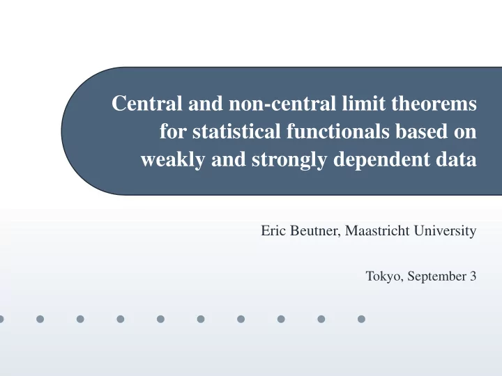
Central and non-central limit theorems for statistical functionals based on weakly and strongly dependent data Eric Beutner, Maastricht University Tokyo, September 3 (atbegshi) Package atbegshi Warning: Ignoring void shipout box Overview
Central and non-central limit theorems for statistical functionals based on weakly and strongly dependent data Eric Beutner, Maastricht University Tokyo, September 3 (atbegshi) Package atbegshi Warning: Ignoring void shipout box
Overview Motivation Motivation Quasi-Hadamard differentiability Quasi-Hadamard differentiability Applications Applications Continuous mapping approach to U- and Continuous mapping approach to U- and V-statistics V-statistics Tokyo, 2013 2
Motivation Statistical functionals Functional delta method Quasi-Hadamard differentiability Applications Motivation Continuous mapping approach to U- and V-statistics Tokyo, 2013 3
Statistical functionals Motivation � Let θ = T ( F ) be some characteristic of the distribution Statistical functionals Functional delta function F (df). method Quasi-Hadamard differentiability Applications Continuous mapping approach to U- and V-statistics Tokyo, 2013 4
Statistical functionals Motivation � Let θ = T ( F ) be some characteristic of the distribution Statistical functionals Functional delta function F (df). method Quasi-Hadamard differentiability � Typical examples are Applications � 0 � ∞ � T ( F ) = − −∞ K ( F ( x )) dx + 0 (1 − K ( F ( x )) dx Continuous mapping approach to U- and so called L-statistics. Distortion risk measures which V-statistics are quite popular are also of this form. Tokyo, 2013 4
Statistical functionals Motivation � Let θ = T ( F ) be some characteristic of the distribution Statistical functionals Functional delta function F (df). method Quasi-Hadamard differentiability � Typical examples are Applications � 0 � ∞ � T ( F ) = − −∞ K ( F ( x )) dx + 0 (1 − K ( F ( x )) dx Continuous mapping approach to U- and so called L-statistics. Distortion risk measures which V-statistics are quite popular are also of this form. � � � T ( F ) = g ( x 1 , x 2 ) dF ( x 1 ) dF ( x 2 ) so called U- or V-statistic (of degree 2). Tokyo, 2013 4
Statistical functionals Motivation � Let θ = T ( F ) be some characteristic of the distribution Statistical functionals Functional delta function F (df). method Quasi-Hadamard differentiability � Typical examples are Applications � 0 � ∞ � T ( F ) = − −∞ K ( F ( x )) dx + 0 (1 − K ( F ( x )) dx Continuous mapping approach to U- and so called L-statistics. Distortion risk measures which V-statistics are quite popular are also of this form. � � � T ( F ) = g ( x 1 , x 2 ) dF ( x 1 ) dF ( x 2 ) so called U- or V-statistic (of degree 2). � Z-estimators. Tokyo, 2013 4
Statistical functionals Motivation � Let θ = T ( F ) be some characteristic of the distribution Statistical functionals Functional delta function F (df). method Quasi-Hadamard differentiability � Typical examples are Applications � 0 � ∞ � T ( F ) = − −∞ K ( F ( x )) dx + 0 (1 − K ( F ( x )) dx Continuous mapping approach to U- and so called L-statistics. Distortion risk measures which V-statistics are quite popular are also of this form. � � � T ( F ) = g ( x 1 , x 2 ) dF ( x 1 ) dF ( x 2 ) so called U- or V-statistic (of degree 2). � Z-estimators. � Given n observations X 1 , . . . , X n with df F a natural estimator is then T ( F n ) with F n the empirical distribution function. Tokyo, 2013 4
Functional delta method Motivation � Well-known: If T is Hadamard differentiable at F , then Statistical functionals Functional delta the asymptotic distribution of T ( F n ) follows immediately method by the (functional) delta method from the asymptotic Quasi-Hadamard differentiability distribution of F n − F . Applications Continuous mapping approach to U- and V-statistics Tokyo, 2013 5
Functional delta method Motivation � Well-known: If T is Hadamard differentiable at F , then Statistical functionals Functional delta the asymptotic distribution of T ( F n ) follows immediately method by the (functional) delta method from the asymptotic Quasi-Hadamard differentiability distribution of F n − F . Applications Continuous mapping � Thus, delta method leads asymptotic distribution of approach to U- and V-statistics T ( F n ) − T ( F ) whenever we have weak convergence of the empirical process. Tokyo, 2013 5
Functional delta method Motivation � Well-known: If T is Hadamard differentiable at F , then Statistical functionals Functional delta the asymptotic distribution of T ( F n ) follows immediately method by the (functional) delta method from the asymptotic Quasi-Hadamard differentiability distribution of F n − F . Applications Continuous mapping � Thus, delta method leads asymptotic distribution of approach to U- and V-statistics T ( F n ) − T ( F ) whenever we have weak convergence of the empirical process. � Many results on weak convergence of the empirical process (iid, short-memory like α -mixing or β -mixing, long memory, etc.). Tokyo, 2013 5
Motivation Quasi-Hadamard differentiability Illustrative example: sample mean Illustrative example: V-statistic Quasi-Hadamard Way out & Problems Quasi-Hadamard differentiability differentiability Quasi-Hadamard differentiability (cont.) Modified FDM Applications Continuous mapping approach to U- and V-statistics Tokyo, 2013 6
Illustrative example: sample mean Motivation � If K corresponds to Lebesgue measure on [0 , 1] , then Quasi-Hadamard differentiability � 0 � ∞ Illustrative example: sample mean − K ( F n ( x )) dx + (1 − K ( F n ( x )) dx, Illustrative example: V-statistic 0 −∞ Way out & Problems Quasi-Hadamard corresponds to the sample mean. differentiability Quasi-Hadamard differentiability (cont.) Modified FDM Applications Continuous mapping approach to U- and V-statistics Tokyo, 2013 7
Illustrative example: sample mean Motivation � If K corresponds to Lebesgue measure on [0 , 1] , then Quasi-Hadamard differentiability � 0 � ∞ Illustrative example: sample mean − K ( F n ( x )) dx + (1 − K ( F n ( x )) dx, Illustrative example: V-statistic 0 −∞ Way out & Problems Quasi-Hadamard corresponds to the sample mean. differentiability Quasi-Hadamard � Proving Hadamard differentiability of this L-statistic (at differentiability (cont.) F ) in the direction of V boils down to prove that Modified FDM � � � � � Applications � � [ V n ( x ) − V ( x )] dx � → 0 , Continuous mapping � approach to U- and V-statistics whenever || V n − V || ∞ → 0 . || · || ∞ denotes sup-norm. Tokyo, 2013 7
Illustrative example: sample mean Motivation � If K corresponds to Lebesgue measure on [0 , 1] , then Quasi-Hadamard differentiability � 0 � ∞ Illustrative example: sample mean − K ( F n ( x )) dx + (1 − K ( F n ( x )) dx, Illustrative example: V-statistic 0 −∞ Way out & Problems Quasi-Hadamard corresponds to the sample mean. differentiability Quasi-Hadamard � Proving Hadamard differentiability of this L-statistic (at differentiability (cont.) F ) in the direction of V boils down to prove that Modified FDM � � � � � Applications � � [ V n ( x ) − V ( x )] dx � → 0 , Continuous mapping � approach to U- and V-statistics whenever || V n − V || ∞ → 0 . || · || ∞ denotes sup-norm. � ⇒ The simplest L-statistic the sample mean is not Hadamard differentiable w.r.t. the sup-norm. Tokyo, 2013 7
Illustrative example: V-statistic Motivation � Proving Hadamard differentiability of a V-statistic (at F ) Quasi-Hadamard differentiability in the direction of V , involves among other things Illustrative example: showing that || V n − V || ∞ → 0 implies sample mean Illustrative example: � � V-statistic Way out & Problems V n ( x 2 ) | dg F | ( x 2 ) → V ( x 2 ) | dg F | ( x 2 ) . Quasi-Hadamard differentiability Quasi-Hadamard differentiability where | dg F | is the absolute measure generated by (cont.) � g F ( x 2 ) = g ( x 1 , x 2 ) dF ( x 1 ) . Modified FDM Applications Continuous mapping approach to U- and V-statistics Tokyo, 2013 8
Illustrative example: V-statistic Motivation � Proving Hadamard differentiability of a V-statistic (at F ) Quasi-Hadamard differentiability in the direction of V , involves among other things Illustrative example: showing that || V n − V || ∞ → 0 implies sample mean Illustrative example: � � V-statistic Way out & Problems V n ( x 2 ) | dg F | ( x 2 ) → V ( x 2 ) | dg F | ( x 2 ) . Quasi-Hadamard differentiability Quasi-Hadamard differentiability where | dg F | is the absolute measure generated by (cont.) � g F ( x 2 ) = g ( x 1 , x 2 ) dF ( x 1 ) . Modified FDM Applications � If g F generates a finite (signed) measure, then || V n − V || ∞ Continuous mapping approach to U- and this implication indeed holds. V-statistics Tokyo, 2013 8
Recommend
More recommend
Explore More Topics
Stay informed with curated content and fresh updates.
