Call-by-value non-determinism in a linear logic type discipline - PowerPoint PPT Presentation

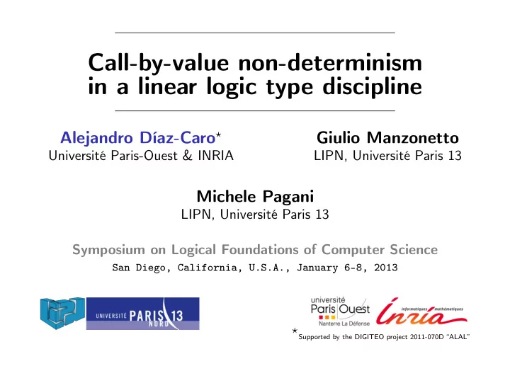
Call-by-value non-determinism in a linear logic type discipline Alejandro Díaz-Caro ⋆ Giulio Manzonetto Université Paris-Ouest & INRIA LIPN, Université Paris 13 Michele Pagani LIPN, Université Paris 13 Symposium on Logical Foundations of Computer Science San Diego, California, U.S.A., January 6–8, 2013 ⋆ Supported by the DIGITEO project 2011-070D “ALAL”

Intersection types discipline [Coppo-Dezani’78] M : α ∩ β M enjoys both properties α and β With this idea in mind intersection is idempotent α ∩ α = α . 2 / 16

Intersection types discipline [Coppo-Dezani’78] M : α ∩ β M enjoys both properties α and β With this idea in mind intersection is idempotent α ∩ α = α . Used to capture various notions of termination: Head, Weak and Strong normalisation [Coppo-Dezani’78, Sallé’80] 2 / 16

Intersection types discipline [Coppo-Dezani’78] M : α ∩ β M enjoys both properties α and β With this idea in mind intersection is idempotent α ∩ α = α . Used to capture various notions of termination: Head, Weak and Strong normalisation [Coppo-Dezani’78, Sallé’80] Resource-aware intersection types [De Carvalho’07] Let us change point of view: M : α ∩ β M will be called once as data of type α and once as data of type β Hence α ∩ α � = α = ⇒ Multisets Used to capture quantitative properties of programs, e.g.: CBN λ -calculus: number of linear head-reduction steps [De Carvalho’07] CBV λ -calculus: number of weak head-reduction steps [Ehrhard’12] 2 / 16

Intersection types discipline [Coppo-Dezani’78] M : α ∩ β M enjoys both properties α and β With this idea in mind intersection is idempotent α ∩ α = α . Used to capture various notions of termination: Head, Weak and Strong normalisation [Coppo-Dezani’78, Sallé’80] Resource-aware intersection types [De Carvalho’07] Let us change point of view: M : α ∩ β M will be called once as data of type α and once as data of type β Hence α ∩ α � = α = ⇒ Multisets Used to capture quantitative properties of programs, e.g.: CBN λ -calculus: number of linear head-reduction steps [De Carvalho’07] CBV λ -calculus: number of weak head-reduction steps [Ehrhard’12] Our goal: extend Ehrhard’s system with non-determinism 2 / 16

May/Must-convergent non-determinism Consider the CBV λ -calculus extended with. . . Non-deterministic choice The machine choses either M or N M + N Parallel composition The machine interleaves reductions in M and in N M � N 3 / 16

May/Must-convergent non-determinism Consider the CBV λ -calculus extended with. . . Non-deterministic choice The machine choses either M or N M + N ◮ The non-deterministic choice M + N is may -convergent: it converges if either M or N converges Parallel composition The machine interleaves reductions in M and in N M � N ◮ The parallel composition M � N is must -convergent: it converges if both M and N do 3 / 16

Λ + � : Its syntax and operational semantics Grammar of Λ + � terms M , N , P , Q ::= V | MN | M + N | M � N Terms: V ::= x | λ x . M Values: Reduction semantics β v -reduction + -reductions � -reductions M + N → M ( M � N ) P → MP � NP ( λ x . M ) V → M [ V / x ] M + N → N V ( M � N ) → VM � VN + Contextual rules selecting the head redex. . . The reduction is lazy (it does not reduce under λ -abstractions) 4 / 16

Λ + � : Its syntax and operational semantics Grammar of Λ + � terms M , N , P , Q ::= V | MN | M + N | M � N Terms: V ::= x | λ x . M Values: Reduction semantics β v -reduction + -reductions � -reductions M + N → M ( M � N ) P → MP � NP ( λ x . M ) V → M [ V / x ] M + N → N V ( M � N ) → VM � VN + Contextual rules selecting the head redex. . . The reduction is lazy (it does not reduce under λ -abstractions) Convergence M → ∗ V 1 � · · · � V n M converges ⇔ 4 / 16

Examples and remarks Application is bilinear op MN + MN ′ + M ′ N + M ′ N ′ ( M + M ′ )( N + N ′ ) ≡ . . . but λ -abstraction is not op λ x . ( M + N ) �≡ λ x . M + λ x . N 5 / 16

Examples and remarks Application is bilinear op MN + MN ′ + M ′ N + M ′ N ′ ( M + M ′ )( N + N ′ ) ≡ . . . but λ -abstraction is not op λ x . ( M + N ) �≡ λ x . M + λ x . N Example of parallel composition and non-deterministic choice ( λ x . ( x � x ))( V + V ′ ) converges to either V � V or V ′ � V ′ ( λ x . ( x + x ))( V � V ′ ) converges to V � V ′ only 5 / 16

Linear logic based type system Translation: Intuitionistic Logic �→ Polarized fragment of LL ι v = ι, ( α → β ) v = α c ⊸ β � , α c = ! α v , α � =? α c Based on [Ehrhard’12] , based on second Girard’s translation. Intuitions from the relational semantics of LL ◮ The type for computations ( · ) c is a multiset [ α v 1 , . . . , α v n ] of value types (representing n calls to a single value of type α v i ), ◮ The type of parallel compositions ( · ) � is another multiset [ α c 1 , . . . , α c n ] of types of each term in the composition, ◮ The type for values ( · ) v are either basic types or functional types, ◮ A functional type in this system is a pair ( α c , [ α c 1 , . . . , α c n ]) . 6 / 16

Linear logic based type system Translation: Intuitionistic Logic �→ Polarized fragment of LL ι v = ι, ( α → β ) v = α c ⊸ β � , α c = ! α v , α � =? α c Based on [Ehrhard’12] , based on second Girard’s translation. Intuitions from the relational semantics of LL ◮ The type for computations ( · ) c is a multiset [ α v 1 , . . . , α v n ] of value types (representing n calls to a single value of type α v i ), ◮ The type of parallel compositions ( · ) � is another multiset [ α c 1 , . . . , α c n ] of types of each term in the composition, ◮ The type for values ( · ) v are either basic types or functional types, ◮ A functional type in this system is a pair ( α c , [ α c 1 , . . . , α c n ]) . Notation First multiset layer − → ⊗ Second multiset layer − → ` Functional type ( α c , [ α c 1 , . . . , α c α c ⊸ α c 1 ` · · · ` α c n ]) − → n Empty computational multiset − → 1 6 / 16

Linear logic based type system (cont.) Grammar of Types: parallel-types: α, β ::= α ` β | τ computational-types: τ, ρ ::= 1 | τ ⊗ ρ | τ ⊸ α � ⊗ tensor product associative and commutative ` par 1 neutral element of ⊗ 7 / 16

Linear logic based type system (cont.) Grammar of Types: parallel-types: α, β ::= α ` β | τ computational-types: τ, ρ ::= 1 | τ ⊗ ρ | τ ⊸ α � ⊗ tensor product associative and commutative ` par 1 neutral element of ⊗ Type environments: Γ = x 1 : τ 1 , . . . , x n : τ n represents the map � τ i if y = x i , Γ( y ) = 1 otherwise. Tensor is extended to environments pointwise (Γ ⊗ ∆)( x ) = Γ( x ) ⊗ ∆( x ) . 7 / 16

Linear logic based type system (cont.) Type inference rules + is may-convergent, so it ∆ ⊢ M : α ∆ ⊢ N : α + ℓ + r is enough that one term is ∆ ⊢ M + N : α ∆ ⊢ M + N : α typable 8 / 16

Linear logic based type system (cont.) Type inference rules + is may-convergent, so it ∆ ⊢ M : α ∆ ⊢ N : α + ℓ + r is enough that one term is ∆ ⊢ M + N : α ∆ ⊢ M + N : α typable ∆ ⊢ M : α 1 Γ ⊢ N : α 2 � I � is must-convergent, so both components must be typable ∆ ⊗ Γ ⊢ M � N : α 1 ` α 2 8 / 16

Linear logic based type system (cont.) Type inference rules + is may-convergent, so it ∆ ⊢ M : α ∆ ⊢ N : α + ℓ + r is enough that one term is ∆ ⊢ M + N : α ∆ ⊢ M + N : α typable ∆ ⊢ M : α 1 Γ ⊢ N : α 2 � I � is must-convergent, so both components must be typable ∆ ⊗ Γ ⊢ M � N : α 1 ` α 2 n i ¸ k ¸ n i � ∆ ⊢ M : ( τ ij ⊸ α ij ) Γ i ⊢ N : τ ij 1 ≤ i ≤ k k ≥ 1 i = 1 j = 1 j = 1 ⊸ E n i ≥ 1 k ¸ k ¸ n i � ∆ ⊗ Γ i ⊢ MN : α ij i = 1 j = 1 i = 1 It reflects the distribution of the parallel operator over the application 8 / 16

Linear logic based type system (cont.) Type inference rules + is may-convergent, so it ∆ ⊢ M : α ∆ ⊢ N : α + ℓ + r is enough that one term is ∆ ⊢ M + N : α ∆ ⊢ M + N : α typable ∆ ⊢ M : α 1 Γ ⊢ N : α 2 � I � is must-convergent, so both components must be typable ∆ ⊗ Γ ⊢ M � N : α 1 ` α 2 n i ¸ k ¸ n i � ∆ ⊢ M : ( τ ij ⊸ α ij ) Γ i ⊢ N : τ ij 1 ≤ i ≤ k k ≥ 1 i = 1 j = 1 j = 1 ⊸ E n i ≥ 1 k ¸ k ¸ n i � ∆ ⊗ Γ i ⊢ MN : α ij i = 1 j = 1 i = 1 It reflects the distribution of the parallel operator over the application ∆ i , x : τ i ⊢ M : α i 1 ≤ i ≤ n n ≥ 0 ⊸ I ax n n � � x : τ ⊢ x : τ ∆ i ⊢ λ x . M : ( τ i ⊸ α i ) i = 1 i = 1 The axiom and the intersection type for values respectively 8 / 16

Examples Γ = y : τ 1 , y ′ : τ 2 ∆ = x : ( τ 1 ⊸ α 1 ) ⊗ ( τ 2 ⊸ α 2 ) Γ ⊢ y � y ′ : τ 1 ` τ 2 ⊸ E ∆ ⊢ x : ( τ 1 ⊸ α 1 ) ⊗ ( τ 2 ⊸ α 2 ) ∆ ⊗ Γ ⊢ x ( y � y ′ ) : α 1 ` α 2 x ( y � y ′ ) → xy � xy ′ 9 / 16