Calibrating Agent-Based Models with Machine Learning Surrogates - PowerPoint PPT Presentation
Calibrating Agent-Based Models with Machine Learning Surrogates Francesco LAMPERTI 1 , 2 , Antoine MANDEL 2 , Andrea ROVENTINI 1 , Amir SANI 2 1 Institute of Economics and LEM, Scuola Superiore SantAnna (Pisa) 2 Universit e Paris 1 Path
Calibrating Agent-Based Models with Machine Learning Surrogates Francesco LAMPERTI 1 , 2 , Antoine MANDEL 2 , Andrea ROVENTINI 1 , Amir SANI 2 1 Institute of Economics and LEM, Scuola Superiore Sant’Anna (Pisa) 2 Universit´ e Paris 1 Path´ eon-Sorbonne, Centre d’Economie de la Sorbonne and CNRS, Paris School of Economics Macroeconomic Agent-Based Modeling Surrogates Workshop February 9th, 2016 Research supported by Horizons 2020 FET, DOLFINS project.
What is the Problem? What is our Approach? Example Evaluation Times Empirical Results Empirical Results
What is the Problem?
( many ) Macroeconomic Agent-Based Models (ABMs) are ◮ computationally expensive ◮ defined by dozens of parameters ◮ hard to calibrate, estimate, test, explore ∗ ∗ Due to complex parameter-specific behaviours.
What are we proposing?
Machine Learning Surrogates !
Faster ◮ Agent-Based Model “Calibration” (e.g. Inference) ◮ Scenario Stress Testing (e.g. Monte Carlo) ◮ Policy Exercises (e.g. Exploration)
Faster ◮ Agent-Based Model “Calibration” (e.g. Inference) ◮ Scenario Stress Testing (e.g. Monte Carlo) ◮ Policy Exercises (e.g. Exploration)
Faster ◮ Agent-Based Model “Calibration” (e.g. Inference) ◮ Scenario Stress Testing (e.g. Monte Carlo) ◮ Policy Exercises (e.g. Exploration)
Surrogate( ABM + “Calibration” Qality Test)
� � Brock & Hommes ABM + Kolmogorov–Smirnov Surrogate Two Sample Test
Brock & Hommes (BH) Very simple ABM with 10 parameters
Brock & Hommes This model is NOT representative of complex Macroeconomic Agent-Based Models
Brock & Hommes Smooth Learning Manifold
but
13.4 quadrillion combinations
Tiny positive region
Enormous parameter space!
The Curse of Dimensionality!
How do we measure calibration quality?
Kolmogorov–Smirnov Two Sample Test (KS)
� � D n , n ′ = sup � F X SP 500 , n ( x ) − F X BH , n ′ ( x ) � � � x
Evaluation Times
Single Evaluation BH + KS = 0 . 30 seconds
Policy Constraint Security prices are not negative
Policy Constraint Only run parameters y i that pass the following constraint (filter), S ( T 1 ∗ P + B 1 ) + ( 1 − S ) ∗ ( T 2 ∗ P + B 2 ) > 0 , where S is the share type, P is the initial deviation from the fundamental price, B 1 and B 2 are the bias of agent 1 and 2, and T 1 and T 2 are the trend of agent 1 and 2.
Simulation X BH ( y i ) = X BH
Simulation Objective y i that produce 250 Log Returns
An obvious Constraint
Length Filter ABM simulations should produce 250 Log Returns
Length Filter len ( X BH ) == 250
Length Filter (Density) 3,000 per 100,000 † † Random Latin Hypercube Sampling[4]
2-Sample KS Test KS ( X SP500 , X BH ) = { D X SP500 , X BH , p-value }
KS Threshold p-value > 0 . 05 D X SP500 , X BH < 0 . 20
KS Threshold (Density) 55 per 1,000,000 ‡ ‡ Random Latin Hypercube Sampling[4]
Dataset Highly Imbalanced!
Evaluation Time
Evaluation Time 1,000,000 samples ≈ 3.5 days
Evaluation Time 100 passing tests ≈ 20.4 days
What about a Machine Learning Surrogate?
Surrogate Modeling ◮ Function Approximation [3] ◮ Meta-Modeling [1] ◮ “Response Surface” Methodology [2, 5] ◮ Experimental Design ◮ Model Emulation ◮ “Model of a Model”
Surrogate Solution • Draw 1 , 000 , 000 parameters using RLH • Policy Constraint ≈ 500 , 000 • Time to compute y PC ≈ 0 . 25 secs i • BH ( y PC ) = X PC : 2 , 500 min i i • Length Constraint ≈ 3 , 000 y PC , len : 5 min i • KS ( X SP 500 , X PC , len , p-value PC , len ) = { D X SP500 , X PC , len } : 800 min i i i • Threshold Constraint ≈ 55 y PC , len , Thresholded : 1 min i
Surrogate Solution • Draw 1 , 000 , 000 parameters using RLH • Policy Constraint ≈ 500 , 000 • Time to compute y PC ≈ 0 . 25 secs i • BH ( y PC ) = X PC : 2 , 500 min i i • Length Constraint ≈ 3 , 000 y PC , len : 5 min i • KS ( X SP 500 , X PC , len , p-value PC , len ) = { D X SP500 , X PC , len } : 800 min i i i • Threshold Constraint ≈ 55 y PC , len , Thresholded : 1 min i
Surrogate Solution • Draw 1 , 000 , 000 parameters using RLH • Policy Constraint ≈ 500 , 000 • Time to compute y PC ≈ 0 . 25 secs i • BH ( y PC ) = X PC : 2 , 500 min i i • Length Constraint ≈ 3 , 000 y PC , len : 5 min i • KS ( X SP 500 , X PC , len , p-value PC , len ) = { D X SP500 , X PC , len } : 800 min i i i • Threshold Constraint ≈ 55 y PC , len , Thresholded : 1 min i
Surrogate Solution • Draw 1 , 000 , 000 parameters using RLH • Policy Constraint ≈ 500 , 000 • Time to compute y PC ≈ 0 . 25 secs i • BH ( y PC ) = X PC : 2 , 500 min i i • Length Constraint ≈ 3 , 000 y PC , len : 5 min i • KS ( X SP 500 , X PC , len , p-value PC , len ) = { D X SP500 , X PC , len } : 800 min i i i • Threshold Constraint ≈ 55 y PC , len , Thresholded : 1 min i
Surrogate Solution • Draw 1 , 000 , 000 parameters using RLH • Policy Constraint ≈ 500 , 000 • Time to compute y PC ≈ 0 . 25 secs i • BH ( y PC ) = X PC : 2 , 500 min i i • Length Constraint ≈ 3 , 000 y PC , len : 5 min i • KS ( X SP 500 , X PC , len , p-value PC , len ) = { D X SP500 , X PC , len } : 4 , 000 min i i i • Threshold Constraint ≈ 55 y PC , len , Thresholded : 1 min i
Total Time BH+KS: 6 , 508 1 4 min
Out of Sample 100 , 000 , 000 out of sample y i § ≈ 2 min § using RLH
BH+KS 1 , 000 × 6 , 508 1 4 min = 6 , 508 , 250 min
Machine Learning Surrogate • ( naive ) Budgeted Model Search ¶ : 60 min ¶ htps://github.com/hyperopt/hyperopt-sklearn
Machine Learning Surrogate Filter OOS using Learned Model ≈ 12 min
Speedup (OOS Only) BH+KS: 1 , 000 × 6 , 508 1 4 min = 6 , 508 , 250 min Machine Learning Surrogate: 72 min ≈ 90 , 392 1 3 × Speedup!
Advantage Reusable Machine Learning Surrogate Model
Thank you!
References [1] Robert W Blanning. The construction and implementation of metamodels. simulation , 24(6):177–184, 1975. [2] George EP Box and KB Wilson. On the experimental atainment of optimum conditions. Journal of the Royal Statistical Society. Series B (Methodological) , 13(1):1–45, 1951. [3] Donald R Jones. A taxonomy of global optimization methods based on response surfaces. Journal of global optimization , 21(4):345–383, 2001. [4] Michael D McKay, Richard J Beckman, and William J Conover. Comparison of three methods for selecting values of input variables in the analysis of output from a computer code. Technometrics , 21(2):239–245, 1979. [5] Raymond H Myers, Douglas C Montgomery, and Christine M Anderson-Cook. Response surface methodology: process and product optimization using designed experiments , volume 705. John Wiley & Sons, 2009. [6] The Art of Sofware. Derivation of Bias-Variance Decomposition , September 2012. http://artofsoftware.org/2012/09/13/ derivation-of-bias-variance-decomposition/ .
Recommend


More recommend
Explore More Topics
Stay informed with curated content and fresh updates.