BRDF Evolution BRDFs have evolved historically 1970s: Empirical - PowerPoint PPT Presentation

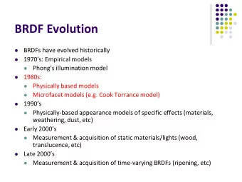
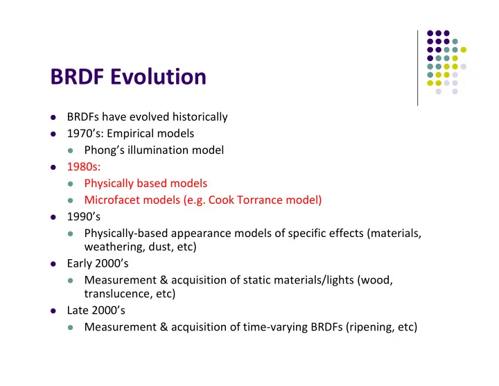
BRDF Evolution BRDFs have evolved historically  1970’s: Empirical models  Phong’s illumination model  1980s:  Physically based models  Microfacet models (e.g. Cook Torrance model)  1990’s  Physically ‐ based appearance models of specific effects (materials,  weathering, dust, etc) Early 2000’s  Measurement & acquisition of static materials/lights (wood,  translucence, etc) Late 2000’s  Measurement & acquisition of time ‐ varying BRDFs (ripening, etc) 

Physically ‐ Based Shading Models  Phong model produces pretty pictures  Cons: empirical (fudged?) ( cos   ), plastic look  Shaders can implement better lighting/shading models  Big trend towards Physically ‐ based lighting models  Physically ‐ based?  Based on physics of how light interacts with actual surface  Apply Optics/Physics theories  Classic: Cook ‐ Torrance shading model (TOGS 1982)

Cook ‐ Torrance Shading Model  Same ambient and diffuse terms as Phong  New, better specular component than ( cos   ),     F , DG    cos   n  v  Where  D ‐ Distribution term  G – Geometric term  F – Fresnel term

Distribution Term, D  Idea: surfaces consist of small V ‐ shaped microfacets (grooves) microfacets Average Incident normal n δ light  Many grooves at each surface point  Grooves facing a direction contribute  D( ) term: what fraction of grooves facing each angle δ δ  E.g. half of grooves at hit point face 30 degrees, etc

Cook ‐ Torrance Shading Model Define angle  as deviation of h from surface normal  Only microfacets with pointing along halfway vector, h = s + v , contributes  n n h    v l l P h P h Can use old Phong cosine ( cos n  ), as D  Use Beckmann distribution instead    2    tan    1     m D ( ) e  2 4 4 m cos ( ) m expresses roughness of surface. How? 

Cook ‐ Torrance Shading Model  m is Root ‐ mean ‐ square (RMS) of slope of V ‐ groove  m = 0.2 for nearly smooth  m = 0.6 for very rough Very smooth Very rough surface surface m is slope of groove

Self ‐ Shadowing (G Term)  Some grooves on extremely rough surface may block other grooves

Geometric Term, G  Surface may be so rough that interior of grooves is blocked from light by edges  Self blocking known as shadowing or masking  Geometric term G accounts for this  Break G into 3 cases:  G, case a: No self ‐ shadowing (light in ‐ out unobstructed)  Mathematically, G = 1

Geometric Term, G  G m , case b: No blocking on entry, blocking of exitting light (masking)   2 ( )( ) n h n h  G  Mathematically,  m h s

Geometric Term, G  G s , case c: blocking of incident light, no blocking of exitting light ( shadowing)  Mathematically,   2 ( n h )( n h )  G  s h s  G term is minimum of 3 cases, hence    1 , , G G m G s

Fresnel Term, F  So, again recall that specular term    ,  F DG  spec   n  v  Microfacets not perfect mirrors  F term, F(  ,  ) gives fraction of incident light reflected     2      2   1 ( ) 1 g c c g c     F is function of material   F 1      2     and incident angle 2 ( g c ) c ( g c ) 1    where c = cos (  ) = n.s and g 2 =  2 + c 2 + 1   is incident angle,  is refractive index of material

Other Physically ‐ Based BRDF Models  Oren ‐ Nayar – Diffuse term changed not specular  Aishikhminn ‐ Shirley – Grooves not v ‐ shaped. Other Shapes  Microfacet generator (Design your own microfacet)

BV BRDF Viewer BRDF viewer (View distribution of light bounce)

BRDF Evolution BRDFs have evolved historically  1970’s: Empirical models  Phong’s illumination model  1980s:  Physically based models  Microfacet models (e.g. Cook Torrance model)  1990’s  Physically ‐ based appearance models of specific effects (materials,  weathering, dust, etc) Early 2000’s  Measurement & acquisition of static materials/lights (wood,  translucence, etc) Late 2000’s  Measurement & acquisition of time ‐ varying BRDFs (ripening, etc) 

Measuring BRDFs Murray ‐ Coleman and Smith Gonioreflectometer. ( Copied and Modified from [Ward92] ).

Measured BRDF Samples  Mitsubishi Electric Research Lab (MERL) http://www.merl.com/brdf/  Wojciech Matusik  MIT PhD Thesis  100 Samples

BRDF Evolution BRDFs have evolved historically  1970’s: Empirical models  Phong’s illumination model  1980s:  Physically based models  Microfacet models (e.g. Cook Torrance model)  1990’s  Physically ‐ based appearance models of specific effects (materials,  weathering, dust, etc) Early 2000’s  Measurement & acquisition of static materials/lights (wood,  translucence, etc) Late 2000’s  Measurement & acquisition of time ‐ varying BRDFs (ripening, etc) 

Time ‐ varying BRDF  BRDF: How different materials reflect light  Time varying?: how reflectance changes over time  Examples: weathering, ripening fruits, rust, etc

Computer Graphics (CS 4731) Lecture 19: Shadows and Fog Prof Emmanuel Agu Computer Science Dept. Worcester Polytechnic Institute (WPI)

Introduction to Shadows  Shadows give information on relative positions of objects Use ambient + diffuse + specular Use just ambient components component

Introduction to Shadows  Two popular shadow rendering methods: Shadows as texture (projection) 1. Shadow buffer 2.  Third method used in ray ‐ tracing (covered in grad class)

Projective Shadows  Oldest method: Used in early flight simulators  Projection of polygon is polygon called shadow polygon Actual polygon Shadow polygon

Projective Shadows  Works for flat surfaces illuminated by point light  For each face, project vertices V to find V’ of shadow polygon  Object shadow = union of projections of faces

Projective Shadow Algorithm  Project light ‐ object edges onto plane  Algorithm:  First, draw ground plane using specular+diffuse+ambient components  Then, draw shadow projections (face by face) using only ambient component

Projective Shadows for Polygon If light is at (x l , y l , z l ) 1. Vertex at (x, y, z) 2. Would like to calculate shadow polygon vertex V projected 3. onto ground at (x p , 0, z p ) (x,y,z) (x p ,0,z p ) Ground plane: y = 0

Projective Shadows for Polygon  If we move original polygon so that light source is at origin  Matrix M projects a vertex V to give its projection V’ in shadow polygon   1 0 0 0   0 1 0 0      M 0 0 1 0   1  0 0 0   y l    

Building Shadow Projection Matrix Translate source to origin with T( ‐ x l , ‐ y l , ‐ z l ) 1. Perspective projection 2. Translate back by T(x l , y l , z l ) 3.   1 0 0 0      1 0 0 x 1 0 0 x   l l     0 1 0 0    0 1 0 y 0 1 0 y        l l M 0 0 1 0        0 0 1 z 0 0 1 z 1 l l      0 0 0      0 0 0 1  0 0 0 1 y     l Final matrix that projects Vertex V onto V’ in shadow polygon

Code snippets?  Set up projection matrix in OpenGL application float light[3]; // location of light mat4 m; // shadow projection matrix initially identity M[3][1] = -1.0/light[1];   1 0 0 0   0 1 0 0      M 0 0 1 0   1  0 0 0   y l    

Projective Shadow Code  Set up object (e.g a square) to be drawn point4 square[4] = {vec4(-0.5, 0.5, -0.5, 1.0} {vec4(-0.5, 0.5, -0.5, 1.0} {vec4(-0.5, 0.5, -0.5, 1.0} {vec4(-0.5, 0.5, -0.5, 1.0}  Copy square to VBO  Pass modelview, projection matrices to vertex shader

What next?  Next, we load model_view as usual then draw original polygon  Then load shadow projection matrix, change color to black, re ‐ render polygon 1. Load modelview draw polygon as usual 2. Modify modelview with Shadow projection matrix Re-render as black (or ambient)

Shadow projection Display( ) Function void display( ) { mat4 mm; // clear the window glClear(GL_COLOR_BUFFER_BIT | GL_DEPTH_BUFFER_BIT); // render red square (original square) using modelview // matrix as usual (previously set up) glUniform4fv(color_loc, 1, red); glDrawArrays(GL_TRIANGLE_STRIP, 0, 4);