Benchmark Problems Wiener Approaches - Coupled Electric Drives - - PowerPoint PPT Presentation

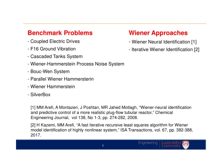
Benchmark Problems Wiener Approaches - Coupled Electric Drives - Wiener Neural Identification [1] - F16 Ground Vibration - Iterative Wiener Identification [2] - Cascaded Tanks System - Wiener-Hammerstein Process Noise System - Bouc-Wen System - Parallel Wiener Hammersterin - Wiener Hammerstein - SilverBox [1] MM Arefi, A Montazeri, J Poshtan, MR Jahed Motlagh, “Wiener-neural identification and predictive control of a more realistic plug-flow tubular reactor,” Chemical Engineering Journal, vol 138, No 1-3, pp. 274-282, 2008. [2] H Kazemi, MM Arefi, “A fast iterative recursive least squares algorithm for Wiener model identification of highly nonlinear system,” ISA Transactions, vol. 67, pp. 382-388, 2017. 1

An Investigation of the Wiener Approach for Nonlinear System Identification Benchmarks Allahyar Montazeri Mohammad Mehdi Arefi, Mehdi Kazemi Lancaster University Faculty of Science and Technology E-mail: a.montazeri@lancaster.ac.uk

Block Oreinted Approach  Physically insightful  Lower number of parameters × The model is not linear in parameters × Difficulty in finding a good initial condition Wiener y n ( ) z n ( ) u n ( ) f x ( ) G q ( ) model structure  Can approximate almost any nonlinear system with high accuracy  No specific assumption on the spectrum input or static nonlinearity 3

Wiener Neural Technique y n ( ) z n ( ) u n ( ) NN x ( ) Estimating the linear part using the given Step 1 input/output data Estimating the nonlinear part (Neural Network) using the estimated linear model and the Step 2 measured output Parametrising the estimated models in the Step 3 previous steps and optimising the overall parameters of the Wiener model

Wiener Neural Technique y n ( ) z n ( ) u n ( ) Step 1 NN x ( )  Assume no non-linear part, input-output data     u n ( ), ( ) : y n n 1 N  Calculate , , A B C D n ( , , , ) x (0)      l               Step 2   NN z n ( ( )) ( , ) s i ( , , ) s i j z n ( ) b s i ( , ) b s ( , 1) ( ) n   j s       i 1 j 1 2      l                ( i s , ) ˆ y ( k ) ( 1 , i ) ( 1 , i , j ) z ( k ) b ( 1 , i ) b ( 1 , 1 )     1 j min    N       i 1 j 1 b ( s , 1 )       θ   l (( l 2 ) 1 )  R θ l        k 1         b ( i s , ) y ( k ) ( l , i ) ( l , i , j ) z ˆ ( k ) b ( l , i ) b ( l , 1 )     l j        i 1 j 1 ( s , i , j )

Wiener Neural Technique y n ( ) z n ( ) u n ( ) Step 3 NN x ( )  Parametrisation of the linear state-space model  Optimising the whole parameters of the system A C Definition- The pair is in the output normal form if ( , )   T T A A C C I n     A C n n l n ,

Wiener Neural Technique  I      C 0   n k T T T     ...   n I      T U ( n l ) ( n l ) 1 2 R A       k k n   I    k 1    S 1 r s       S T T U k k k t s s , r 1 t , I s s .   k T k k k k k k l k k   r s t k k k        U l 1 ( l 1) ( l 1) s 1, s k k k s parameter vector k θ Initial condition x (0) on 2 N  The parameters in  θ θ ˆ min y k ( ) y k ( , , ) B D ( , ) matrices on θ θ x (0), ,  on k 1 θ NN parameters

Wiener Neural Technique  Levenberg-Marquardt to optimize the whole parameters 2   y  Θ  ˆ Θ θ θ min y ( ) 2 0 Θ    Θ Θ ΔΘ ( t 1 ) ( t ) ( t ) Nonlinear SYS ID  Θ y ˆ ( ( )) t in SLICOT    J θ i : , i 1: N j , 1: length ( ).  Software ij Θ j  Θ ˆ ( ( )) y t    L θ i : , i 1: N j , length ( ).  ij Θ j  J  L  0 0 1 1   J  L 0 0    J 2 2      J J I Θ J Θ T T ( ( t ) ( t ) ) e ( ( t ))           J L   0 0 l l

Benchmark Criteria  A plot with the modelled output and the simulation error in time domain  A plot of simulation error in frequency domain N 1      ˆ e y k ( ) y k ( ) mean N  t 1 N 1      2 ˆ e y k ( ) y k ( ) rms N  t 1  ˆ y y    FIT (1 ) 100  y y J. Schoukens, J. Suykens, L. Ljung, “Wiener-Hammerstein Benchmark,” 15th IFAC Symposium on System Identification (SYSID 2009) , July 6-8, St. Malo, France, 2009.

SilverBox System  A second order mechanical system with nonlinear stiffness.        2 k y ( ) a by my dy k y y ( ) u Input/output data  First part: filtered white Gaussian signal 10 realisation of Filtered with cut off frequency 200Hz. multi-sine signal Gaussian Noise  Second part: odd harmonic multi-sine with uniformly distributed random phase.  High SNR. Input Estimation data  ID1 filtered white Gaussian (1:40,000)  ID2 multi-sine (80,000:126,000)  ID3 mixed of ID1 and ID2 (1:100,000) Output Test data  TST1 130,000:188,000  TST2 126,000:188,000

SilverBox Parameters Neural network order = 10 State space model order = 5 Parameter s = 20 ID2-TST2 Silver Box System TEST TST1 TST2 ESTM Residu ID1 MEAN 2.4e ‐ 4 2.5e ‐ 5 RMS 3e ‐ 3 4.5e ‐ 3 FIT 66.2% 84.1% ID2 MEAN 1.2e ‐ 4 1.3e ‐ 4 RMS 2.2e ‐ 3 3.1e ‐ 3 Residu (dB) FIT 74% 89.1% Residual error ID3 MEAN 2e ‐ 4 2.1e ‐ 4 spectrum RMS 2.4e ‐ 3 3.3e ‐ 3 FIT 71.8% 88.4%

Winer-Hammerstein System y n ( ) x n ( ) w n ( ) u n ( )  f x ( ) 3 rd order Chebyshev filter with cut G q 2 ( ) G q 1 ( ) off 4.4 kHz  3 rd order inverse Chebyshev filter with cut off 5kHz  Transmission zero in the frequency Test data band of interest Estimation data Input/Output test data  Filtered Gaussian signal with cut off 10kHz  Sampling frequency 51.2kHz  SNR 70dB

Winer-Hammerstein State space model order = 6 Parameter s = 15 Test Neural network order = 15 Residu Residu (dB) Residual error spectrum

Winer-Hammerstein Pole-Zero Map 1 0.8 0.6 0.4 Imaginary Axis 0.2 Mag(dB) 0 -0.2 -0.4 -0.6 -0.8 -1 -1 -0.5 0 0.5 1 1.5 2 2.5 Real Axis Frequency response plot of the Pole-Zero map linear part of the linear part P1= 0.89 � i0.17 NOTE: transmission zero of the second P2=0.7 � i0.4 filter is captured Z1= 0.6 � i0.99 Z2= 0.8 � i0.6

Wiener-Hammerstein with Noise e n ( ) x u n ( ) Input/Output estimation data y n ( ) w n ( ) G q 1 ( ) G q 2 ( ) f x ( )  Multi-sine input up to 15kHz (2 periods, x n ( ) e n ( ) 1 amplitude, 4096 points per period) y e n ( )  u Additive process noise (filtered white u ( ) n y ( ) n Gaussian, cut off 20kHz ) m m  Additive measurement noise (white Gaussian noise) Test data Estimation data  Test data Noiseless multi-sine and swept sine input input output output

Winer-Hammerstein with Noise FIT = -0.89747 % State space model order = 5 2 Measured Output Model Output 1 Parameter s = 15 Test 0 Neural network order = 15 -1 -2 0 200 400 600 800 1000 1200 1400 1600 1800 2000 rms= 0.7169, mean = 0.017049 2 1 Residu 0 -1 Residu (dB) -2 2000 4000 6000 8000 10000 12000 14000 16000 Samples Residual error spectrum

Winer-Hammerstein with Noise Imaginary Axis Mag(dB) Frequency response plot of the Pole-Zero map linear part of the linear part P= 0.94 � i0.11 Z1= 0.58 � i0.84 Z2= 1 � i0.36

Iterative Least Square Wiener  ( ) n C q ( ) A q ( )  d m n ( ) q B q ( ) y n ( ) x n ( ) u n ( ) f x ( ) A q ( )  b q       1 n d B q ( ) b b q q B q ( ) b  0 1 n x n ( ) u n ( ) b A q ( )  a q      1 n A q ( ) 1 a q a 1 n a  m n ( ) f x n ( ( ))  c q      1 n C q ( ) 1 c q c 1 n c C q ( )  A q   y n ( ) ( ) n m n ( )        n  2 f x ( ) x x x f ( ) 1 2 n f