Bayesian Neural Networks - Presenters Group 1: A Practical Bayesian - PowerPoint PPT Presentation
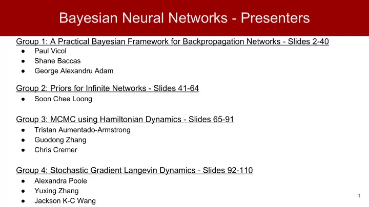
Bayesian Neural Networks - Presenters Group 1: A Practical Bayesian Framework for Backpropagation Networks - Slides 2-40 Paul Vicol Shane Baccas George Alexandru Adam Group 2: Priors for Infinite Networks - Slides 41-64
Bayesian Approach over Architectures ○ P(T) ~ N(E[T|X=x^(m)], ● Probabilistic assumptions on the random variables of interest: 1/ß) i.e. the r.v. T where corresponds to particular with ○ ● E[T|X=x^(m)] ≈ y(x^(m), w, A) additive Gaussian noise ○ the random vector is Gaussian with mean 0 and precision parameter ○ P( w ) ~ N(0, 1/\alpha) ● This implies: Gaussian Integrals Prior: Likelihood: Posterior: 25
Finding the Posterior ● The posterior is given by ● Finding the most probable value of for the posterior, i.e., is equivalent to minimizing the regularized cost function , defined as , for But how do we find the parameters and ? 26
MacKay Bayesian Framework By Bayes Theorem: We assign a uniform prior to and and have Now let and Evaluate integrals directly Now let: N:= |D|*|dim(t^(m))| & k = dim( w ) For we must use Laplace approximation for 27 Gaussian integrals
Estimating and for NNs ● Assume: ○ The posterior probability of and consists of well separated islands in parameter space each centered around a minimum of ● Consider a minimum of and define the solution as the ensemble of networks A in the neighborhood of and all symmetric permutations of that ensemble. ● Posterior probability of solution is: where 28
How do we Calculate ? ● We have expressions for every quantity but ; because of our assumption, we can use Laplace approximation: |D|/dim(x^(m)) ● Where is the Hessian of evaluated at ● This approximation works when is “large” by C.L.T. ● Also: ○ Recent paper from Pennington and Bahri (JMLR, 2017) also treats Hessian estimation for NNs using Random Matrix Theory 29
Comparing Models ● To assign preference to alternative architectures and regularizers, we evaluate the evidence of the solutions we found by marginalizing out and : ● It is important to note we do NOT need the posterior of and over the entire set of possible architectures (this would be computationally infeasible) ● Instead we wish to compare pre-trained NNs which have found their own minimum and rank them in some objective manner
Evidence and Generalization Error Evidence and Generalization Error ● Evidence and generalization error are correlated ● But evidence is not always a good predictor of generalization error ○ Validation error is noisy, and requires a large held-out dataset ○ If two models yield identical regression results, their gen errors are the same, but evidence may differ due to model complexity (penalized by the Occam factor) 31
Model Complexity and Generalization Error Image from: Hastie, T. et al., Elements of Statistical Learning. Springer . p. 38. 2013. Train Error Test Error
Evidence - Occam Hill Evidence - Occam Hill Occam hill Occam factor Evidence vs Num Hidden Units 33
Comparing Models ● The second last slide showed us that using training error on its own will lead to overfitting and poor generalization ● The red circled region shows models with good generalization but low evidence ● This contradicts what we thought Bayesian model comparison does ● We must be missing something! Test Error vs Log Evidence
Failure as an Opportunity to Learn Failure as an Opportunity to Learn ● What if the evidence is low , but generalization error is good (low)? ○ i.e., we have poor correlation between evidence and gen error ● Then the model likely does not match the real world ● Learn from the failure: Check and evaluate model assumptions, try new models until one achieves better fit with the data ○ This is a benefit of using Bayesian methods; from gen error, can’t discover the inconsistency between the model and data 35
Inconsistent Prior ● Our loss function is standard, so let’s look at our prior more closely ● Suppose we rescale the inputs ● Our prior is inconsistent Then we could rescale the weights in the first Net B does the same thing yet the prior penalizes Net B more than Net A layer and end up with the same mapping Original figure by G. A. Adam
Adjusting the Prior ● The previous prior assumed dependence in the scale of the weights between layers ● Let’s use a prior that has independent regularizing constants for each layer: ● Notice how the bottom left region of high evidence but poor generalization no longer exists
Overview Summary from Neal ● Variance of the Gaussian prior for the weights and biases is a hyperparameter ○ Allows the model to adapt to the degree of smoothness indicated by the data ● Improved by using several variance hyperparameters, one for each type of parameter (input-to-hidden weights, hidden biases, and output weights/biases) ● This emphasizes the advantages of hierarchical models ● Makes sense: Network inputs and outputs are different quantities with different scales; using a single variance hyperparameter depends on arbitrary choice of measurement units. 38
Conclusion ● Bayesian evidence is in fact a good predictor of generalization ability ● Combined with generalization error, it can help us determine if we are using an inconsistent regularizer and change our worldview ● Evidence is maximized for neural nets with reasonable numbers of hidden units ● Computational difficulty arises in calculating the Hessian, its inverse, and determinant ● This framework is also applicable to classification problems ○ Error landscape would look totally different since we would be using different loss functions
References ● Blundell, C. et al. Weight Uncertainty in Neural Networks. ICML 37, 1613-1622, 2015. ● MacKay, D. Information Theory, Inference, and Learning Algorithms . Cambridge University Press. 2003. ● MacKay, D. A Practical Bayesian Framework for Backpropagation Networks. Neural Computation 4 , 448-472, 1992. ● MacKay, D. Bayesian Interpolation. Neural Computation 4 , 415-447, 1992. ● Laplace Approximation. https://en.wikipedia.org/wiki/Laplace%27s_method. Retrieved September 25, 2017. ● Pennington, J. and Bahri, Y. Geometry of Neural Network Loss Surfaces via Random Matrix Theory. PMLR 70 , 2798-2806, 2017.
Priors for Infinite Networks Based on: Chapter 2 of Bayesian Learning for Neural Networks By: Radford M. Neal Presented by: Soon Chee Loong
Overview Distributions over Weights and Functions ● The weights of a network determine the function computed by the network ● In a BNN, the weights are drawn from a probability distribution ; intuitively, we can interpret the BNN as representing a distribution over functions ● The first step in Bayesian inference is the specification of a prior e.g., a prior over weights, ○ ● Given a prior over the weights, what is the prior over computed functions? ● Connection between bayesian neural networks and Gaussian Processes 42
Overview Overview ● How do we decide priors for neural networks? ● A single hidden layer neural network with infinite hidden units converges to a Gaussian Process. ● A single hidden layer neural network with infinite hidden units approaches a limiting distribution . ● The choice of hidden function activation influences the type of functions sampled from the prior. ● Not covered from Radford’s Chapter 2 Thesis: Hierarchical Models 43
Overview Motivation: Selecting Priors ● Prior represents our beliefs about the problem. Recap: Coin toss problem, heads and tails with 50% probability makes sense to us. ○ Solve problem due to M.L.E. with coin toss by introducing uniform priors. ■ ● Neural Networks ○ priors over weights/biases has no obvious connection to input. ● The use of infinite networks makes sense from the standpoint of prior beliefs ○ We usually don’t believe that the function we want to learn can be perfectly captured by a finite network. ● Properties of gaussian priors for infinite networks can be found analytically. 44
Overview Motivation: Bigger is Better ● Bayesian Occam Razor: Bayesian approach: ○ can increase model parameters to infinity without overfitting. ● In practice, limited by computational resources (memory, time) ● NOT restricted based on size of training set. ● Wouldn’t we overfit? No, if we regularize it properly. Analogous to Neural Networks: ○ “Make network as big as possible” ■ ■ “Then, regularize using weight decay, dropout.” (Jimmy Ba, ECE521 2017 Lecture) ● What should we increase in Neural Networks to Infinity? 45
Universal Approximation Theorem. Overview ● Universal Approximation Theorem: ○ can approximate any continuous function with a neural network with 1 hidden layer. ● Hence, focus on extending hidden layer to infinite number of hidden units. ● Assumption: Computationally feasible to produce mathematically correct results for infinite hidden units. 46 - Online Open Access Textbooks, 9.3 Neural Network Models
What Priors to Use Overview ● Since no obvious connection, what priors do we use? ● Gaussian with zero mean is standard. ● Historically by David Mackay, ○ Gaussian with zero mean has worked well for his work. Minimize standard deviation of priors as a form of regularization. ○ Similar to weight decay for neural networks. ■ 47 - Natural Resource Biometrics, NR3110
Overview Infinite Networks → Gaussian Processes ● Consider a Bayesian Neural Network with a single hidden layer: input-to-hidden hidden-to-output ● Examine the prior distribution on the output . value for a fixed input . O I . We want to find 48 Original figure by P. Vicol H
Overview Output Variance Limit Behavior Without Regularization ● Behavior of output ● Total Variance ○ Central Limit Theorem - Bishop, Pattern Recognition and Machine Learning Need to get rid of dependence on H 49
Overview Output Variance Limit Behavior With Regularization ● Reduce initialization variance as form of regularization 50
Overview Output Variance With Regularization Output variance finite! 51
Overview Output Variance With Regularization Proof works for any zero mean, finite variance prior distribution. Output variance finite! 52
Overview Priors Converge to Gaussian Process ● Similarly, (mathematical proof for Prior Joint Distribution) ● Gaussian Priors converge to Gaussian Process as number of hidden units increases. 53
Functions Drawn Approaches Limiting Distribution Overview (From CSC2541 2017: Lecture 2 pg. 36 of 55) 54
Functions Drawn From Prior Distribution Overview With Step(z) Hidden Activation Approaches Limiting Distribution H = 300 H = 10000 Converges Converges Converges Converges 55 - Radford Neal, PhD Thesis, Chapter 2
Overview Priors to Brownian or Smooth Function ● How does Hidden Unit Activation affect output function sampled? ○ h(z) = sign(z) h(z) = tanh(z) ○ ● Gaussian Prior with zero mean. ● Priors properties are determined by the covariance function. ○ Smooth ○ Fractional Brownian ○ Brownian 56
Overview Priors that Lead to Brownian Functions ● Let input-to-hidden weights and hidden biases have Gaussian distributions -1 ● Step activations 1 -0.8 ● The function is built up of small, 0.5 independent, non-differentiable 0.5 1 . steps contributed by hidden units. 0.2 . . ● Brownian 0.5 1 0.7 57 Original figure by P. Vicol
Overview Priors that Lead to Smooth Functions ● Let input-to-hidden weights and hidden biases have Gaussian distributions -0.3 ● Tanh activations 1 -0.8 ● The function is built up of small, 0.5 independent, differentiable tanh 0.5 0.45 . contributed by hidden units 0.2 . . ● Smooth 0.5 0.95 0.7 58
Overview Priors that Lead to Smooth and Brownian Functions - Radford Neal, PhD Thesis, Chapter 2 Gaussian priors, step() hidden units Gaussian priors, tanh() hidden units 59
Tanh(): Smooth Converges to Brownian Overview as the prior over the mean increases to infinity - Radford Neal, PhD Thesis, Chapter 2 Gaussian priors, hidden units 60
Overview Priors to Brownian or Smooth Function ● Behavior is based on Covariance Function ● Re-write covariance function in terms of the differences. 61
Overview Prior over Function Covariance Properties ● Priors properties are determined by the covariance function. ○ Smooth ■ ○ Fractional Brownian ■ ○ Brownian ■ 62 - Radford Neal, PhD Thesis, Chapter 2
Non Gaussian Prior (Cauchy) Overview with Step Hidden Activation Non-Gaussian Prior Gaussian Prior with Step() (Cauchy) with Step() Large jumps from single hidden unit. 63 - Radford Neal, PhD Thesis, Chapter 2
Overview GPs vs NNs ● When would we use NNs vs GPs? ● GPs are just “smoothing devices” (MacKay, 2003) ○ Are NNs over-hyped, or are GPs underestimated? (MacKay says both .) Neural Networks Gaussian Processes ● Simple matrix operations on the ● Optimizing parameters of a network covariance matrix of the GP ● Can solve many problems not solvable by ● GPs are easy to implement and use - few GPs: e.g., representation learning parameters must be specified by hand ● Inverting an NxN matrix is expensive - Can’t scale to large datasets (N > 1000) 64
Hamiltonian Monte Carlo Based on: MCMC using Hamiltonian Dynamics by Radford Neal Presented by: Tristan Aumentado-Armstrong, Guodong Zhang, Chris Cremer
Markov Chain Monte Carlo (MCMC) I ● Recall: in Bayesian analysis, we often desire integrals like (Posterior Predictive Dist.) (Expectation of y=f(x|θ)) ● But how can we actually evaluate these integrals when θ is very high dimensional? Use Markov Chain Monte Carlo (MCMC), which is much less affected by dimensionality. 66
Markov Chain Monte Carlo (MCMC) II ● Monte Carlo is a way of performing this integration, by transforming the problem in the following way: where θ i is distributed according to the posterior for the parameters, P(θ|D) ● This transforms our integral into a sampling problem, so that we now just need a way to sample from the posterior 67
The Metropolis-Hastings (MH) Algorithm I ● MH is an MCMC algorithm for sampling from the posterior P(θ|D) ● Intuition: Run a Markov chain with stationary distribution P(θ|D) ● Algorithm (Assume: Q(θ) � P(θ|D)) ○ Start from initial state θ 0 ○ Iterate i = 1 to n: ■ Propose: ■ Acceptance Probability 68
The Metropolis-Hastings (MH) Algorithm II ● Given enough time, MH converges to sampling from the stationary distribution ○ At this point, states are samples from the posterior (as desired) ● Common proposal choice: Random Walk MH ○ The proposal perturbs the current state (e.g. Gaussian noise) and is symmetric ○ The new proposed state is accepted/rejected based on how likely the parameters are according to the posterior Murray, MCMC Slides, Machine Learning Summer School 2009 69
The Metropolis-Hastings (MH) Algorithm III ● This accept-reject step ensures that the state update (transition) satisfies the equations of detailed balance where is the state transition probability ● Such chains are reversible , which is desirable for MCMC algorithms Reversibility can be used to show the MCMC updates don’t alter Q ○ This is sufficient for the chain’s stationary distribution to exist and, in this case, ○ equal our posterior by construction 70
The Metropolis-Hastings (MH) Algorithm IV ● Choosing a proposal distribution: e.g. ○ Balance exploration (reach areas with support) & visiting high probability areas more ○ Control the random walk step size with � Too large: too many rejections ■ Too small: explores the space too slowly ■ ● Drawbacks of the Random Walk MH Algorithm ○ The algorithm may find it very difficult to move long distances in parameter space ■ Random walks are not very efficient explorers ○ If � is too large or small, then the samples will be too dependent (lower effective sample size) ● We want a way to move larger distances, yet still have a decent chance of acceptance - Idea: prefer moving along level sets of an energy related to Q 71
Hamiltonian Monte Carlo - Motivation ● For MCMC, the distribution we wish to sample can be related to a potential energy function via the concept of canonical distribution from statistical mechanics Canonical distribution ● We can draw samples from canonical distribution using random walk Metropolis ( guess-and-check ). But it cannot produce distant proposals with high acceptance probability. 72
Hamiltonian Monte Carlo - Motivation ● The key here is to exploit additional information to guide us through the neighborhood with high target probability. Gradient !!! image credit: A Conceptual introduction to Hamiltonian Monte Carlo
Hamiltonian Monte Carlo - Motivation ● Following along the gradient would pulls us towards the mode of the target density . We lose the chance to explore new and unexplored areas. Momentum !!! image credit: A Conceptual introduction to Hamiltonian Monte Carlo
Hamiltonian energy ● Introduce the momentum (where is variable of interest, say position) ● We can now lift up the target distribution onto a joint distribution ● By the definition of canonical distribution, the expanded system defines a Hamiltonian energy that decomposes into a potential energy and kinetic energy. Note: for convenience, I just use one-dimensional notations in my slide.
Hamiltonian dynamics ● Hamiltonian dynamics describe how kinetic energy is converted to potential energy (and vice versa) as a particle moves throughout a system in time. ● This description is implemented quantitatively via a set of differential equations known as the Hamilton’s equations : ● These equations define a mapping from to
Property - Reversibility Property 1: For the mapping from to , we can find inverse mapping by first negating , applying , and negating again. negate negate Note: Detailed balance requires each transition is reversible. 77
Property - Hamiltonian Conservation Property 2: Hamiltonian H doesn’t have a functional dependence on time. It’s invariant over time. Note: In practice, Hamiltonian is approximately invariant.
Property - Volume Preservation Property 3: In Hamiltonian dynamics, any contraction or expansion in position space must be compensated by a respective expansion or compression in momentum space. A B Sufficient and necessary condition: the determinant of Jacobian matrix of the mapping having absolute value one
Leave target distribution invariant ● Hamiltonian Conservation ● Reversibility ● Volume Preservation
Discretizing Hamilton’s equations ● For computer implementation, Hamilton’s equations must be approximated by discretizing time, using some small stepsize, . ● The best known way to approximate the solution is Euler’s method ● Euler’s method is not volume preserving and not reversible. image credit: MCMC using Hamiltonian dynamics
Leapfrog method https://en.wikipedia.org/wiki/Shear_mapping Note: each step is “shear” transformation which is volume preservation.
Accept / Reject ● In practice, using finite stepsizes will not preserve the Hamiltonian exactly and will introduce bias in the simulation. image credit: MCMC using Hamiltonian dynamics ● HMC cancels these effects exactly by adding a Metropolis accept/reject stage, after n leapfrog steps, the proposed state will be accepted with the probability , defined as 83
Summary ● Sample momentum from its canonical distribution ● Perform n leapfrog steps and obtain the proposed state ● Accept/reject the proposed state 84
MH vs HMC Metropolis-Hastings Hamiltonian Monte Carlo ● Initialize x ● Initialize x ● For s=1,2...N: ● For s=1,2...N: ○ Sample momentum v = N(0,M) ○ Sample from proposal x’ ~ q(x’|x) ○ Simulate Hamiltonian dynamics x’,v’ = LF(x,v) ○ Accept sample with probability: ○ Accept sample with probability: min(1, p(x’,v’)/p(x,v)) min(1, p(x’)q(x|x’)/p(x)q(x’|x)) ○ If accept: ○ If accept: x = x’ x = x’ ○ Else: ○ Else: x = x x = x
Visualization ● MH: https://chi-feng.github.io/mcmc-demo/app.html#RandomWalkMH,banana ● HMC: https://chi-feng.github.io/mcmc-demo/app.html#HamiltonianMC,banana 86
HMC - Bayesian Perspective ● Goal: Sample x ~ p(x) ○ Construct Markov chain p(x’|x) Want: ○ ■ High acceptance probability: p(x’)/p(x) (more efficient, less rejections) ■ Distant proposals: x’ far from x (better mixing) ● Introduce auxiliary variable v and integrate it out ○ x ~ p(x) = /int p(x,v) (sampling momentum) Chain becomes: p(x’,v’|x,v) ○ ○ Acceptance becomes: p(x’,v’)/p(x,v) ■ This ratio can stay high while x’ can be very different than x ■ Hamiltonian dynamics achieves the desired properties 87
How do we know we’re sampling the correct distribution? ● Detailed Balance (sufficient but not necessary) Why: Metropolis-Hastings Hamiltonian Monte Carlo 88
HMC for BNNs ● Radford Neal Thesis - Chapter 3 Exploration Experiment Y-axis: square root of the Proposal Acceptance average squared magnitude Solid: .1 76% of the hidden-output weights Dotted: .3 39% Dashed: .9 4% X-axis: super-transitions (2000 steps) HMC .3 87% 89
Data Sub-Sampling in MCMC ● Problem: ○ Computing likelihood for MH acceptance step requires the whole dataset ○ For HMC, also need gradient of whole dataset ● Stochastic Gradient HMC (2014) ● Towards scaling up Markov chain Monte Carlo: an adaptive subsampling approach (2014) ● Austerity in MCMC Land: Cutting the Metropolis-Hastings Budget (2014) 90
References ● MCMC & MH Introduction/Tutorials ○ Neal, Bayesian Learning for Neural Networks, Chapter 1, 1995 ○ Robert, The Metropolis-Hastings Algorithm, 2016 ○ Yildirim, Bayesian Inference: Metropolis-Hastings Sampling, 2012 91
Stochastic Gradient Langevin Dynamics Based on: Bayesian Learning via Stochastic Gradient Langevin Dynamics By: Max Welling, Yee Whye Teh Bayesian Dark Knowledge By: Balan et al. Presented by: Alexandra Poole, Yuxing Zhang, Jackson K-C Wang 92
Overview ● Bayesian learning for small mini-batches Bridging optimization and Bayesian learning ✫ ■ Recall Lecture 1: learning MAP versus learning the posterior distribution ● Simple framework that transitions from optimization to posterior sampling ● 2 perspectives on the algorithm ○ Adding Gaussian noise to Stochastic Gradient Descent (SGD) updates ○ Mini-batch Langevin Dynamics (LD) ● This paper is not ○ just proposing a new optimizer 93
Langevin Dynamics Bayesian Learning Full Batch GD Langevin Dynamics ● Langevin Dynamics is used for the proposal step in Metropolis-adjusted Langevin Algorithm(MALA) ○ MALA is a technique of MCMC (proper posterior sampling technique) ● Only a slight modification of Full Batch GD ○ Injects Gaussian noise to parameter updates The reject/accept step from the classic MALA framework is dropped here, because when epsilon is small enough, the acceptance rate approaches 1. 94
Langevin Dynamics MALA : animation ● ○ Href: https://chi-feng.github.io/mcmc-demo/app.html#MALA,banana ○ Why is having a small stepsize important in this paper? (try it!) ■ Notice how when stepsize is reduced, the acceptance rate goes up! 95
SGD Optimization Full Batch GD Mini Batch GD (SGD) In SGD, at each iteration t, update is performed based on a subset of data, ● approximating the true gradient over the whole dataset ● N, and n can differ by orders of magnitude (e.g. 128 vs 1,000,000) ○ In practice, optimization of NN (non-Bayesian) appears to take a long time (large number of iterations ), but it usually translates to <50 passes over the full dataset ( epoch ). ○ But 50 samples for MCMC is definitely not enough 96
SGLD Full Batch GD Langevin Dynamics Mini Batch GD (SGD) SGLD 97
Visually speaking… The figures are actually animations in the presentation. Please visit: https://github.com/wangkua1/SGLD-presentation-supp/tree/master 98
99
Justify SGLD ● What approximation is SGLD making to MALA, and why is it still valid MCMC? ○ First approximation: when epsilon is small enough, the accept/reject is ignored ○ Second approximation: using subsampled gradient to approximate true gradient Let’s rewrite SGLD Approximately recovers LD 100
Recommend
More recommend
Explore More Topics
Stay informed with curated content and fresh updates.
