Bayes rule recall def of conditional: P(a|b) = P(a^b) / P(b) if - PDF document

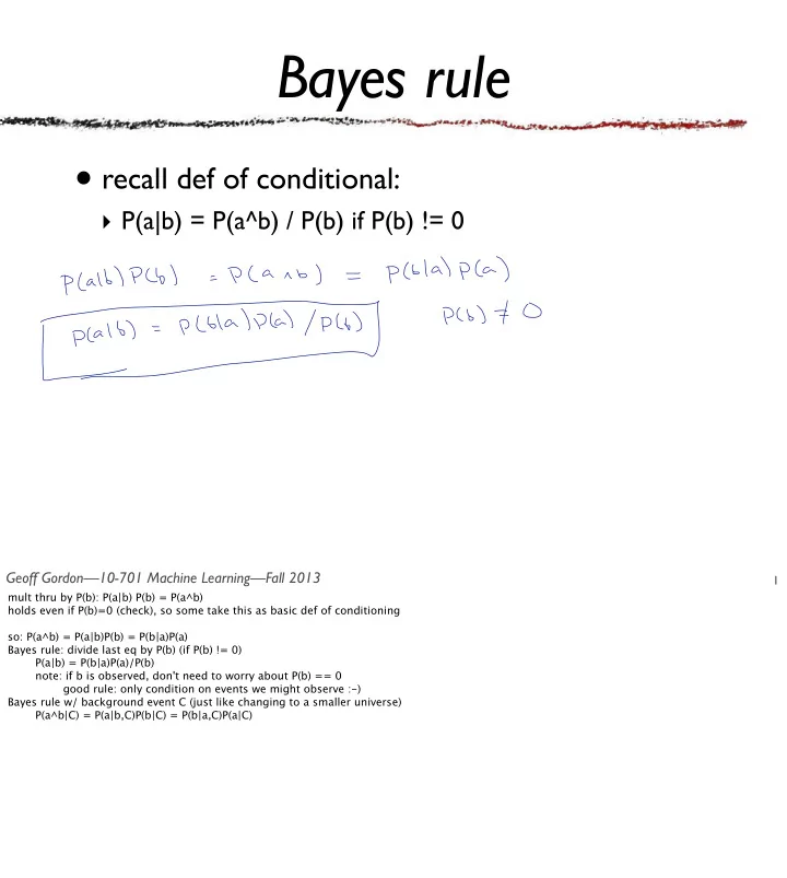
Bayes rule • recall def of conditional: ‣ P(a|b) = P(a^b) / P(b) if P(b) != 0 ‣ Geoff Gordon—10-701 Machine Learning—Fall 2013 1 mult thru by P(b): P(a|b) P(b) = P(a^b) holds even if P(b)=0 (check), so some take this as basic def of conditioning so: P(a^b) = P(a|b)P(b) = P(b|a)P(a) Bayes rule: divide last eq by P(b) (if P(b) != 0) P(a|b) = P(b|a)P(a)/P(b) note: if b is observed, don't need to worry about P(b) == 0 good rule: only condition on events we might observe :-) Bayes rule w/ background event C (just like changing to a smaller universe) P(a^b|C) = P(a|b,C)P(b|C) = P(b|a,C)P(a|C)

Bayes rule: sum version • P(a | b) = P(b | a) P(a) / P(b) Geoff Gordon—10-701 Machine Learning—Fall 2013 2 what if we don't know P(b), but still know P(b|a) and P(a) (often happens) suppose MEEP A = a1, a2, ..., an for moderate n we know sum_i P(ai | b) = 1 so sum_i P(ai | b) P(b) = P(b) (mult by P(b) on both sides) LHS is sum_i P(b|ai) P(ai) (another application of Bayes rule) each term assumed known, sum tractable since n moderate

Bayes rule in ML • P(model | data) = P(data | model) P(model) / P(data) Geoff Gordon—10-701 Machine Learning—Fall 2013 3 Why do we care about Bayes? Lets us take info about conditional in one direction (P(data | model)) and get info about the other direction (P(model| data)). LHS P(model|data) tells us which models are probable give the data. This is (mostly) what we want out of ML! Called “posterior” P(data | model) usually has an explicit formula, e.g., gaussian distribution: P(x_i|mu) = exp(-(x_i-mu)^2/2)/ √ 2pi). Called “likelihood” P(model) = “prior” -- sometimes controversial but not hard to write a minimally reasonable one P(data): “normalizing constant” (also “annoyance”) -- often hard to get can use sum version of Bayes rule (sum numerator over models) OK if not too many models under consideration can use sum version + approximation tricks (numerical quadrature, MCMC like Gibbs) another idea on next slide note: normalizing constants are often ignored. This is a common pattern, but it doesn’t mean it’s always safe (or a good idea) to ignore them! Sometimes all of the useful information is in the normalizing constant...

Bayes rule vs. MAP vs. MLE • P(model | data) = P(data | model) P(model) / P(data) Geoff Gordon—10-701 Machine Learning—Fall 2013 4 MAP: just take model for which RHS is highest -- if we have to choose just one point from posterior density, why not this one? [sketch] now P(data) really is ignorable (doesn’t change order) Seems like a horrible approximation (from Bayesian perspective), but actually has theory to back it up. MLE: ignore P(model) term too. Why? Because people argue about the prior; because with enough evidence from data it might become negligible. Seems even worse, but still has theory to back it up. (see next slide)

Frequentist vs. Bayes see also: http://www.xkcd.com/1132/ FIGHT!!! rev. Thomas Bayes Jerzy Neyman • Nature as adversary vs. Nature as probability distribution • Probability as long-run frequency of repeatable events vs. odds for bets I'm willing to take Geoff Gordon—10-701 Machine Learning—Fall 2013 5 treat Nature as a probability distribution vs. an adversary Bayes: if you have the right distribution over models and can compute with it, good things happen Frequentist: but both of those are horrible assumptions Plenty of paradoxes for both sides if you want to cast stones

Test for a rare disease • About 0.1% of all people are infected • Test detects all infections • Test is highly specific: 1% false positive • You test positive. What is the probability you have the disease? Geoff Gordon—10-701 Machine Learning—Fall 2013 6 P(disease) P(test | +disease) P(test | -disease) P(+disease | +test) = P(+test | +disease) P(+disease) / P(+test) P(+t) = P(+t|+d)P(+d) + P(+t|-d)P(-d) = 1 * .001 / (1*.001 + .01*.999) = .091

Test for a rare disease • About 0.1% of all people are infected • Test detects all infections Bonus: what is probability an average med student • Test is highly specific: 1% false positive gets this question wrong? • You test positive. What is the probability you have the disease? Geoff Gordon—10-701 Machine Learning—Fall 2013 6 P(disease) P(test | +disease) P(test | -disease) P(+disease | +test) = P(+test | +disease) P(+disease) / P(+test) P(+t) = P(+t|+d)P(+d) + P(+t|-d)P(-d) = 1 * .001 / (1*.001 + .01*.999) = .091

Follow-up test • Test 2: detects 90% of infections, 5% false positives ‣ P(+disease | +test1, +test2) = Geoff Gordon—10-701 Machine Learning—Fall 2013 7 P(+disease | +test1, +test2) = P(+1, +2 | +d) P(+d) / P(+1, +2) P(+12) = P(+12|+d)P(+d) + P(+12|-d)P(-d) = 1*.9*.001 / (1*.9*.001 + .05*.01*.999) = .643 Test 1 seems better than test 2 -- why not use test 1 twice? A: T1 is conditionally independent of T2 given disease state -- probably not true for T1 w/ itself

Independence Geoff Gordon—10-701 Machine Learning—Fall 2013 8 for events: defined as P(a^b) = P(a)P(b), like rows/cols of checkerboard P(~a^b) = P(b) – P(a^b) = P(b) - P(a)P(b) = (1-P(a))P(b) = P(~a)P(b) for r.v.s: P(A,B) = P(A)P(B) shorthand: joint probability table = outer product of marginal probability tables P(A=a_i ^ B=b_i) = P(A=a_i) P(B=b_i) intuition: knowing a or ~a tells us nothing about B Bayes rule version: P(A) = P(A|B) i.e., P(A=a_i) = P(A=a_i | B=b_j) for all a_i, b_j w/ P(B=b_j > 0) follows: P(a|b) = P(a^b)/P(b) = P(a)P(b)/P(b) = P(a), as long as P(b)!=0 some take this as definition of independence

Conditional independence Geoff Gordon—10-701 Machine Learning—Fall 2013 9 conditional independence: X _|_ Y | Z if, for all values of z_i, P(X,Y|z_i)=P(X|z_i)P(Y|z_i) i.e., after we condition on z_i, X and Y are independent P(x, y | z) = P(x | z) P(y | z) for any values xyz of XYZ this is a statement about a 3d table and two 2d tables

Conditionally Independent London taxi drivers: A survey has pointed out a positive and significant correlation between the number of accidents and wearing coats. They concluded that coats could hinder movements of drivers and be the cause of accidents. A new law was prepared to prohibit drivers from wearing coats when driving. Finally another study pointed out that people wear coats when it rains… slide credit: Barnabas

More on the importance of conditioning humor credit: xkcd Geoff Gordon—10-701 Machine Learning—Fall 2013 11

Samples … Geoff Gordon—10-701 Machine Learning—Fall 2013 12 i.i.d. sample of an r.v.: N independent copies of the same checkerboard sample is itself an r.v. in a bigger space (a 2N-dim hypercheckerboard) atomic events are tuples of original atomic events sample (r.v.) vs. population (the One True checkerboard) statistic = any function of the sample usu. order-independent (symmetric) but doesn't have to be statistics are r.v.s e.g., sample mean, variance goal of statistics (big or small S): use statistics to find out something about the population

Recall: spam filtering Geoff Gordon—10-701 Machine Learning—Fall 2013 13 classification problem: given data (x_i, y_i) N pairs, x_i \in {0,1}^d, y_i \in {0,1} -- write x_i = (x_{i1} .. x_{id}) produce rule which goes from future x -> predicted y e.g.: spam filtering: x_ij = presence of word i in doc j bag of words

Bag of words Geoff Gordon—10-701 Machine Learning—Fall 2013 14

A ridiculously naive assumption • Assume: • Clearly false: • Given this assumption, use Bayes rule Geoff Gordon—10-701 Machine Learning—Fall 2013 15 assumption: x_{ij} _|_ x_{ik} | c_i for all j,k \in 1..d, j != k clearly false: "CMU" not independent of "Bayes" given this "naive" assumption, use "Bayes" rule

Graphical model spam spam . . . x i x 1 x 2 x n i=1..n Geoff Gordon—10-701 Machine Learning—Fall 2013 16 arrows spam-> xi say xi depends on spam lack of other arrows into xi: the xi’s are conditionally independent given spam “macro” or “for loop” shorthand: called a “plate model”

Naive Bayes • P(spam | email ∧ award ∧ program ∧ for ∧ internet ∧ users ∧ lump ∧ sum ∧ of ∧ Five ∧ Million) Geoff Gordon—10-701 Machine Learning—Fall 2013 17 P(spam | email award program for internet users lump sum of Five Million) = P(email ... Million | spam) P(spam) / [P(email ... Million | spam) P(spam) + P(email ... Million | not-spam) P(~spam)] (sum version of Bayes rule) = P(email | spam) P(award | spam) ... P(Million | spam) P(spam) / [ "" | spam + "" | ~spam] (independence assumption) suppose we know P(word j | spam) and P(word j | ~spam) for all j and suppose we know P(spam) and P(~spam) how? see slightly later then above is easy to calculate! now keep messages w/ P(spam) < threshold adjust threshold based on user preference: chance of missing internet lottery win vs. wants to get work done

In log space z spam = ln(P(email | spam) P(award | spam) ... P(Million | spam) P(spam)) z ~spam = ln(P(email | ~spam) ... P(Million | ~spam) P(~spam)) Geoff Gordon—10-701 Machine Learning—Fall 2013 18 z_spam = ln(P(email | spam) P(award | spam) ... P(Million | spam) P(spam)) z_~spam = ln(P(email | ~spam) P(award | ~spam) ... P(Million | ~spam) P(~spam)) result is then P(spam | ... ) = exp(z_spam) / [exp(z_spam) + exp(z_~spam)] = 1 / [1 + exp(z_~spam - z_spam)] = 1 / [1 + exp(-z)] where z = z_spam - z_~spam sigmoid or logistic function (sketch): logit(z) big z: confident in spam big -z: confident in ~spam