Background: assess the demand Y existing around a service (i.e. - PowerPoint PPT Presentation

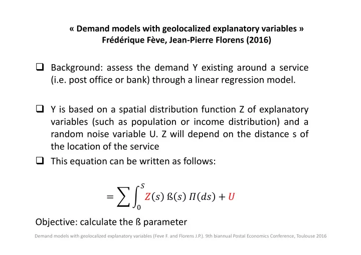
« Demand models with geolocalized explanatory variables » Frédérique Fève, Jean ‐ Pierre Florens (2016)  Background: assess the demand Y existing around a service (i.e. post office or bank) through a linear regression model.  Y is based on a spatial distribution function Z of explanatory variables (such as population or income distribution) and a random noise variable U. Z will depend on the distance s of the location of the service  This equation can be written as follows: � � � � � � ß � � �� � � � Objective: calculate the ß parameter Demand models with geolocalized explanatory variables (Feve F. and Florens J.P.). 9th biannual Postal Economics Conference, Toulouse 2016

Z and U exogeneous: E(Z,U)=0 Calculation of the regularisation parameter α of ß α through Tikhonov • regularisation: � 2 α = arg min �yi � � zi, ß α �2� �� �� � � ��� • ß estimation through Tikhonov regularisation with optimal α => β estimated and β actual curves very similar Demand models with geolocalized explanatory variables (Feve F. and Florens J.P.). 9th biannual Postal Economics Conference, Toulouse 2016

Z and U endogeneous: E(Z,U) ≠ 0 Instrumental variable W introduced • Calculation of the regularisation parameter α of ß α through Tikhonov • regularisation ß estimation through Tikhonov regularisation with optimal α • => β estimated and β actual curves less similar Demand models with geolocalized explanatory variables (Feve F. and Florens J.P.). 9th biannual Postal Economics Conference, Toulouse 2016

Comments & Questions  Interesting approach to analyse demand of a specific service with a relevant implementation on public hospitals  Use of strong methods in econometrics and analysis carried out in a systematic manner  Should be clearer as to why both cases (exogeneity and endogeneity) have been considered  Rather concerned about using euclidean distance s on the simulation in urban area rather than travel time or generalised cost (car or public transport) as results must be significantly different especially in peak periods  Why does the hospital capacity curve show a second peak at km 45 ‐ 50 in a urban zone? Demand models with geolocalized explanatory variables (Feve F. and Florens J.P.). 9th biannual Postal Economics Conference, Toulouse 2016