Axiomatic Foundations of Multiplier Preferences Tomasz Strzalecki - PowerPoint PPT Presentation
Axiomatic Foundations of Multiplier Preferences Tomasz Strzalecki Multiplier preferences Expected Utility inconsistent with observed behavior We (economists) may not want to fully trust any probabilistic model. Hansen and Sargent:
Axiomatic Foundations of Multiplier Preferences Tomasz Strzalecki
Multiplier preferences Expected Utility inconsistent with observed behavior We (economists) may not want to fully trust any probabilistic model. Hansen and Sargent: “robustness against model misspecification”
Multiplier preferences Unlike many other departures from EU, this is very tractable: Monetary policy – Woodford (2006) Ramsey taxation – Karantounias, Hansen, and Sargent (2007) Asset pricing: – Barillas, Hansen, and Sargent (2009) – Kleshchelski and Vincent (2007)
Multiplier preferences But open questions: → Where is this coming from? What are we assuming about behavior (axioms)?
Multiplier preferences But open questions: → Where is this coming from? What are we assuming about behavior (axioms)? → Relation to ambiguity aversion (Ellsberg’s paradox)?
Multiplier preferences But open questions: → Where is this coming from? What are we assuming about behavior (axioms)? → Relation to ambiguity aversion (Ellsberg’s paradox)? → What do the parameters mean (how to measure them)?
Sources of Uncertainty
Ellsberg Paradox
Ellsberg Paradox
Ellsberg Paradox
Ellsberg Paradox
Ellsberg Paradox
Ellsberg Paradox
Ellsberg Paradox
Ellsberg Paradox
Sources of Uncertainty
Sources of Uncertainty
Sources of Uncertainty
Sources of Uncertainty Small Worlds (Savage, 1970; Chew and Sagi, 2008) Issue Preferences (Ergin and Gul, 2004; Nau 2001) Source-Dependent Risk Aversion (Skiadas)
Main Result Within each source (urn) multiplier preferences are EU
Main Result Within each source (urn) multiplier preferences are EU But they are a good model of what happens between the sources
Criterion
Savage Setting S – states of the world Z – consequences f : S → Z – act
Expected Utility u : Z → R – utility function q ∈ ∆( S ) – subjective probability measure
Expected Utility u : Z → R – utility function q ∈ ∆( S ) – subjective probability measure V ( f ) = – Subjective Expected Utility
Expected Utility u : Z → R – utility function q ∈ ∆( S ) – subjective probability measure V ( f ) = f s – Subjective Expected Utility
Expected Utility u : Z → R – utility function q ∈ ∆( S ) – subjective probability measure V ( f ) = u ( f s ) – Subjective Expected Utility
Expected Utility u : Z → R – utility function q ∈ ∆( S ) – subjective probability measure � V ( f ) = S u ( f s ) d q ( s ) – Subjective Expected Utility
Multiplier preferences q – reference measure (best guess)
Multiplier preferences � V ( f ) = u ( f s ) d p ( s ) q – reference measure (best guess)
Multiplier preferences � V ( f ) = min p ∈ ∆( S ) u ( f s ) d p ( s ) q – reference measure (best guess)
Multiplier preferences � V ( f ) = min p ∈ ∆( S ) u ( f s ) d p ( s ) + θ R ( p � q ) q – reference measure (best guess)
Multiplier preferences � V ( f ) = min p ∈ ∆( S ) u ( f s ) d p ( s ) + θ R ( p � q ) Kullback-Leibler divergence relative entropy: � d p � � R ( p � q ) = log d p d q q – reference measure (best guess)
Multiplier preferences � V ( f ) = min p ∈ ∆( S ) u ( f s ) d p ( s ) + θ R ( p � q ) q – reference measure (best guess)
Multiplier preferences � V ( f ) = min p ∈ ∆( S ) u ( f s ) d p ( s ) + θ R ( p � q ) θ ∈ (0 , ∞ ] θ ↑⇒ model uncertainty ↓ θ = ∞ ⇒ no model uncertainty q – reference measure (best guess)
Observational Equivalence When only one source of uncertainty Link between model uncertainty and risk sensitivity: Jacobson (1973); Whittle (1981); Skiadas (2003) dynamic multiplier preferences = (subjective) Kreps-Porteus-Epstein-Zin
Observational Equivalence Multiplier Criterion EU Criterion � → u and θ not identified → Ellsberg’s paradox cannot be explained
Observational Equivalence � − u � � − exp for θ < ∞ , θ φ θ ( u ) = for θ = ∞ . u
Observational Equivalence � − u � � − exp for θ < ∞ , θ φ θ ( u ) = for θ = ∞ . u φ θ ◦ u is more concave than u more risk averse
Observational Equivalence Dupuis and Ellis (1997) � � � � u ( f s ) d p ( s ) + θ R ( p � q ) = φ − 1 φ θ ◦ u ( f s ) d q ( s ) min θ p ∈ ∆ S S S
Observational Equivalence Observation (a) If � has a multiplier representation with ( θ, u , q ), then it has a EU representation with ( φ θ ◦ u , q ).
Observational Equivalence Observation (a) If � has Observation (b) If � has a multiplier representation a EU representation with with ( θ, u , q ), then it has a ( u , q ), where u is bounded EU representation with from above, then it has ( φ θ ◦ u , q ). a multiplier representation with ( θ, φ − 1 ◦ u , q ) for any θ θ ∈ (0 , ∞ ].
Boundedness Axiom Axiom There exist z ≺ z ′ in Z and a non-null event E , such that wEz ≺ z ′ for all w ∈ Z
Enriching the Domain: Two Sources
Enriching Domain f : S → Z – Savage act (subjective uncertainty) ∆( Z ) – lottery (objective uncertainty) f : S → ∆( Z ) – Anscombe-Aumann act
Anscombe-Aumann Expected Utility f s ∈ ∆( Z ) u ( f s ) = � ¯ z u ( z ) f s ( z )
Anscombe-Aumann Expected Utility f s ∈ ∆( Z ) u ( f s ) = � ¯ z u ( z ) f s ( z ) � V ( f ) = u ( f s ) d q ( s ) ¯ S
Axiomatization
Variational Preferences Multiplier preferences are a special case of variational preferences � V ( f ) = min u ( f s ) d p ( s ) + c ( p ) ¯ p ∈ ∆( S ) axiomatized by Maccheroni, Marinacci, and Rustichini (2006) Multiplier preferences: � V ( f ) = min u ( f s ) d p ( s ) + θ R ( p � q ) ¯ p ∈ ∆( S )
MMR Axioms A1 (Weak Order) The relation � is transitive and complete
MMR Axioms A2 (Weak Certainty Independence) For all acts f , g and lotteries π, π ′ and for any α ∈ (0 , 1) α f + (1 − α ) π � α g + (1 − α ) π � α f + (1 − α ) π ′ � α g + (1 − α ) π ′
MMR Axioms A3 (Continuity) For any f , g , h the sets { α ∈ [0 , 1] | α f + (1 − α ) g � h } and { α ∈ [0 , 1] | h � α f + (1 − α ) g } are closed
MMR Axioms A4 (Monotonicity) If f ( s ) � g ( s ) for all s ∈ S , then f � g
MMR Axioms A5 (Uncertainty Aversion) For any α ∈ (0 , 1) f ∼ g ⇒ α f + (1 − α ) g � f
MMR Axioms A6 (Nondegeneracy) f ≻ g for some f and g
MMR Axioms Axioms A1-A6 � Variational Preferences
MMR Axioms A7 (Unboundedness) There exist lotteries π ′ ≻ π such that, for all α ∈ (0 , 1), there exists a lottery ρ that satisfies either π ≻ αρ + (1 − α ) π ′ or αρ + (1 − α ) π ≻ π ′ . A8 (Weak Monotone Continuity) Given acts f , g , lottery π , sequence of events { E n } n ≥ 1 with E n ↓ ∅ f ≻ g ⇒ π E n f ≻ g for large n
MMR Axioms Axioms A1-A6 � Variational Preferences Axiom A7 ⇒ uniqueness of the cost function c ( p ) Axiom A8 ⇒ countable additivity of p ’s.
Axioms for Multiplier Preferences
P2 (Savage’s Sure-Thing Principle) For all events E and acts f , g , h , h ′ : S → Z ⇒ fEh ′ � gEh ′ fEh � gEh =
P2 (Savage’s Sure-Thing Principle) For all events E and acts f , g , h , h ′ : S → Z ⇒ fEh ′ � gEh ′ fEh � gEh =
P4 (Savage’s Weak Comparative Probability) For all events E and F and lotteries π ≻ ρ and π ′ ≻ ρ ′ ⇒ π ′ E ρ ′ � π ′ F ρ ′ π E ρ � π F ρ =
P4 (Savage’s Weak Comparative Probability) For all events E and F and lotteries π ≻ ρ and π ′ ≻ ρ ′ ⇒ π ′ E ρ ′ � π ′ F ρ ′ π E ρ � π F ρ =
P6 (Savage’s Small Event Continuity) For all Savage acts f ≻ g and π ∈ ∆( Z ), there exists a finite partition { E 1 , . . . , E n } of S such that for all i ∈ { 1 , . . . , n } f ≻ π E i g and π E i f ≻ g .
Main Theorem Axioms A1-A8, together with P2, P4, and P6, are necessary and sufficient for � to have a multiplier representation ( θ, u , q ). Moreover, two triples ( θ ′ , u ′ , q ′ ) and ( θ ′′ , u ′′ , q ′′ ) represent the same multiplier preference � if and only if q ′ = q ′′ and there exist α > 0 and β ∈ R such that u ′ = α u ′′ + β and θ ′ = αθ ′′ .
Proof Idea
Proof: Step 1 � on lotteries → identify u (uniquely) � � MMR axioms → V ( f ) = I u ( f ) ¯ I defines a preference on utility acts x , y : S → R x � ∗ y iff I ( x ) ≥ I ( y ) Where I ( x + k ) = I ( x ) + k for x : S → R and k ∈ R (Like CARA, but utility effects, rather than wealth effects)
Recommend
More recommend
Explore More Topics
Stay informed with curated content and fresh updates.
