AvramParter and Szeg o limit theorems: from weak convergence to - PowerPoint PPT Presentation
AvramParter and Szeg o limit theorems: from weak convergence to uniform approximation Egor A. Maximenko based on joint works with Johan Manuel Bogoya, Albrecht B ottcher, and Sergei M. Grudsky Instituto Polit ecnico Nacional, ESFM,
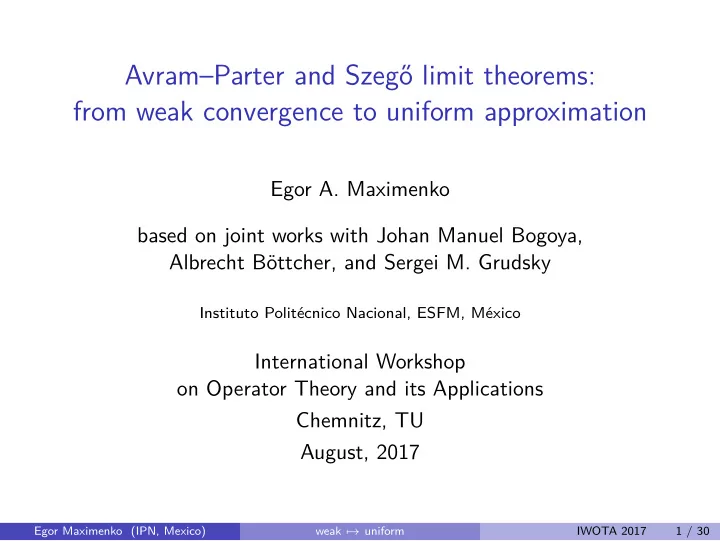
Avram–Parter and Szeg˝ o limit theorems: from weak convergence to uniform approximation Egor A. Maximenko based on joint works with Johan Manuel Bogoya, Albrecht B¨ ottcher, and Sergei M. Grudsky Instituto Polit´ ecnico Nacional, ESFM, M´ exico International Workshop on Operator Theory and its Applications Chemnitz, TU August, 2017 Egor Maximenko (IPN, Mexico) weak �→ uniform IWOTA 2017 1 / 30
Szeg˝ o’s first limit theorem and other theorems about asymptotic distribution can be turned inside out. Egor Maximenko (IPN, Mexico) weak �→ uniform IWOTA 2017 2 / 30
Szeg˝ o’s first Quantile limit theorem function Uniform convergence Egor Maximenko (IPN, Mexico) weak �→ uniform IWOTA 2017 3 / 30
Szeg˝ o’s first Quantile limit theorem function Uniform convergence Egor Maximenko (IPN, Mexico) weak �→ uniform IWOTA 2017 4 / 30
Toeplitz matrices a 0 a − 1 a − 2 a − 3 a − 4 a 1 a 0 a − 1 a − 2 a − 3 T 5 ( a ) = a 2 a 1 a 0 a − 1 a − 2 . a 3 a 2 a 1 a 0 a − 1 a 4 a 3 a 2 a 1 a 0 It is convenient to think that a k are the Fourier coefficients of a certain function a defined on [0 , 2 π ]: � 2 π a k = 1 a ( θ ) e − ki θ d θ. 2 π 0 The function a is called the generating symbol of the matrices � n T n ( a ) = � a j − k j , k =1 . Egor Maximenko (IPN, Mexico) weak �→ uniform IWOTA 2017 5 / 30
Hermitian Toeplitz matrices, real bounded symbols We suppose that the generating symbol is bounded and real: a ∈ L ∞ ([0 , 2 π ] , R ) . The corresponding Toeplitz matrices are Hermitian: a − k = a k , a 0 ∈ R . a 0 a 1 a 2 a 3 a 4 a 1 a 0 a 1 a 2 a 3 T 5 ( a ) = . a 2 a 1 a 0 a 1 a 2 a 3 a 2 a 1 a 0 a 1 a 4 a 3 a 2 a 1 a 0 The spectra of T n ( a ) “asymptotically fill” [ ess inf ( a ) , ess sup ( a )]: ess inf ( a ) ≤ λ ( n ) ≤ . . . ≤ λ ( n ) ≤ ess sup ( a ) , 1 n sp( T n ( a )) → [ ess inf ( a ) , ess sup ( a )] (in Hausdorff distance) . Egor Maximenko (IPN, Mexico) weak �→ uniform IWOTA 2017 6 / 30
Behavior of the eigenvalues of Hermitian Toeplitz matrices Graph of a Eigenvalues of T 8 ( a ) 1 1 0 0 π 2 π Egor Maximenko (IPN, Mexico) weak �→ uniform IWOTA 2017 7 / 30
Behavior of the eigenvalues of Hermitian Toeplitz matrices Graph of a Eigenvalues of T 16 ( a ) 1 1 0 0 π 2 π Egor Maximenko (IPN, Mexico) weak �→ uniform IWOTA 2017 7 / 30
Behavior of the eigenvalues of Hermitian Toeplitz matrices Graph of a Eigenvalues of T 32 ( a ) 1 1 0 0 π 2 π Egor Maximenko (IPN, Mexico) weak �→ uniform IWOTA 2017 7 / 30
Behavior of the eigenvalues of Hermitian Toeplitz matrices Graph of a Eigenvalues of T 32 ( a ) 1 1 β =0 . 4 how many? α =0 . 1 0 0 π 2 π First question: How many eigenvalues are in [ α, β ] ? Egor Maximenko (IPN, Mexico) weak �→ uniform IWOTA 2017 7 / 30
Behavior of the eigenvalues of Hermitian Toeplitz matrices Graph of a Eigenvalues of T 32 ( a ) 1 1 λ (32) ≈ ? 20 0 0 π 2 π First question: How many eigenvalues are in [ α, β ] ? λ ( n ) Second question: ≈ ? j Egor Maximenko (IPN, Mexico) weak �→ uniform IWOTA 2017 7 / 30
Szeg˝ o’s first limit theorem (1920) generating symbol test function a ∈ L ∞ ([0 , 2 π ] , R ) ϕ ∈ C ( R ) � 2 π n 1 1 ϕ ( λ ( n ) � ) − − − → ϕ ( a ( θ )) d θ j n 2 π 0 j =1 Egor Maximenko (IPN, Mexico) weak �→ uniform IWOTA 2017 8 / 30
Another form of the Szeg˝ o’s first limit theorem generating symbol α < β a ∈ L ∞ ([0 , 2 π ] , R ) a ( θ ) � = α, β a.e. # { j : α ≤ λ ( n ) µ R ( a − 1 ([ α, β ])) ≤ β } j − − − → n 2 π Egor Maximenko (IPN, Mexico) weak �→ uniform IWOTA 2017 9 / 30
Another form of the Szeg˝ o’s first limit theorem distribution of the eigenvalues of Hermitian Toeplitz matrices generating symbol v ∈ R a ∈ L ∞ ([0 , 2 π ] , R ) a ( θ ) � = v a.e. # { j : λ ( n ) ≤ v } µ R ( { θ ∈ [0 , 2 π ]: a ( θ ) ≤ v } ) j − − − → n 2 π Egor Maximenko (IPN, Mexico) weak �→ uniform IWOTA 2017 10 / 30
Example to illustrate Szeg˝ o’s first limit theorem Graph of a Eigenvalues of T 32 ( a ) 1 1 0 . 4 0 0 2 π Egor Maximenko (IPN, Mexico) weak �→ uniform IWOTA 2017 11 / 30
Example to illustrate Szeg˝ o’s first limit theorem Graph of a Eigenvalues of T 32 ( a ) 1 1 0 . 4 15 eigenvalues 0 0 2 π 15 32 ≈ 0 . 469 Egor Maximenko (IPN, Mexico) weak �→ uniform IWOTA 2017 11 / 30
Example to illustrate Szeg˝ o’s first limit theorem Graph of a Eigenvalues of T 32 ( a ) 1 1 0 . 4 15 eigenvalues 0 0 2 π 15 32 ≈ 0 . 469 Egor Maximenko (IPN, Mexico) weak �→ uniform IWOTA 2017 11 / 30
Example to illustrate Szeg˝ o’s first limit theorem Graph of a Eigenvalues of T 32 ( a ) 1 1 0 . 4 15 eigenvalues 0 0 2 π 15 32 ≈ 0 . 469 Egor Maximenko (IPN, Mexico) weak �→ uniform IWOTA 2017 11 / 30
Example to illustrate Szeg˝ o’s first limit theorem Graph of a Eigenvalues of T 32 ( a ) 1 1 0 . 4 15 eigenvalues 0 0 2 π µ R { θ : a ( θ ) ≤ 0 . 4 } 15 = 0 . 483 32 ≈ 0 . 469 2 π Egor Maximenko (IPN, Mexico) weak �→ uniform IWOTA 2017 11 / 30
Szeg˝ o found an approximate answer to the first question: how many eigenvalues belong to a given interval? The second question was still open: λ ( n ) ≈ ? j Egor Maximenko (IPN, Mexico) weak �→ uniform IWOTA 2017 12 / 30
Szeg˝ o’s first Quantile limit theorem function Uniform convergence Egor Maximenko (IPN, Mexico) weak �→ uniform IWOTA 2017 13 / 30
Definition of the quantile function BPM ( R ) := Borel probability measures over R . Given µ ∈ BPM ( R ), one defines: the cumulative distribution function F µ : R → [0 , 1], F µ ( v ) := µ ( −∞ , v ] , Egor Maximenko (IPN, Mexico) weak �→ uniform IWOTA 2017 14 / 30
Definition of the quantile function BPM ( R ) := Borel probability measures over R . Given µ ∈ BPM ( R ), one defines: the cumulative distribution function F µ : R → [0 , 1], F µ ( v ) := µ ( −∞ , v ] , the quantile function Q µ : (0 , 1) → R , Q µ ( p ) := inf { v ∈ R : F µ ( v ) ≥ p } , Egor Maximenko (IPN, Mexico) weak �→ uniform IWOTA 2017 14 / 30
Definition of the quantile function BPM ( R ) := Borel probability measures over R . Given µ ∈ BPM ( R ), one defines: the cumulative distribution function F µ : R → [0 , 1], F µ ( v ) := µ ( −∞ , v ] , the quantile function Q µ : (0 , 1) → R , Q µ ( p ) := inf { v ∈ R : F µ ( v ) ≥ p } , and the support of µ : supp( µ ) := { v ∈ R : ∀ ε > 0 µ ( v − ε, v + ε ) > 0 } . Egor Maximenko (IPN, Mexico) weak �→ uniform IWOTA 2017 14 / 30
Quantile function associated to a list of real numbers X = ( − 1 , 0 . 6 , 1 . 1) . Associate the weight 1 / 3 to each one of the elements of X : µ ( {− 1 } ) = µ ( { 0 . 6 } ) = µ ( { 1 . 1 } ) = 1 3 . The corresponding cdf and the quantile function: 1 . 1 1 0 . 6 2 / 3 1 / 3 0 1 2 1 3 3 − 1 0 0 . 6 1 . 1 − 1 Egor Maximenko (IPN, Mexico) weak �→ uniform IWOTA 2017 15 / 30
Quantile function associated to a list of real numbers 118 100 195 166 164 123 102 172 164 117 The same numbers in the ascending order ( α 1 ≤ α 2 ≤ . . . ≤ α 10 ): 100 102 117 118 123 164 164 166 172 195 Q α (1 / 3) = α ⌈ 10 / 3 ⌉ = α 4 = 118. Q α ( p ) = α ⌈ np ⌉ . Egor Maximenko (IPN, Mexico) weak �→ uniform IWOTA 2017 16 / 30
Quantile function associated to a function Let a ∈ L ∞ ([0 , 2 π ] , R ). Pushforward measure µ ∈ BPM ( R ): µ ( B ) := 1 2 πµ R ( a − 1 ( B )) . F a := the cumulative distribution function of a : F a ( v ) := 1 2 π µ R { θ ∈ [0 , 2 π ]: a ( θ ) ≤ v } , v ∈ R . Q a := the corresponding quantile function : Q a ( p ) := inf { v ∈ R : F a ( v ) ≥ p } , p ∈ (0 , 1) . Egor Maximenko (IPN, Mexico) weak �→ uniform IWOTA 2017 17 / 30
Construction of the quantile function associated to a piecewise-linear real function Graph of a 1 3 4 1 4 0 π π 3 π 2 π 2 2 Egor Maximenko (IPN, Mexico) weak �→ uniform IWOTA 2017 18 / 30
Construction of the quantile function associated to a piecewise-linear real function Graph of a 1 3 4 1 4 0 π π 3 π 2 π 2 2 Egor Maximenko (IPN, Mexico) weak �→ uniform IWOTA 2017 18 / 30
Construction of the quantile function associated to a piecewise-linear real function Graph of a 1 1 3 3 4 4 1 1 4 4 0 π π 3 π 2 π 0 19 11 1 2 48 16 2 Egor Maximenko (IPN, Mexico) weak �→ uniform IWOTA 2017 18 / 30
Construction of the quantile function associated to a piecewise-linear real function Graph of a Graph of Q a 1 1 1 3 3 3 4 4 4 1 1 1 4 4 4 0 π π 3 π 2 π 0 19 11 1 19 11 1 0 2 48 16 2 48 16 Egor Maximenko (IPN, Mexico) weak �→ uniform IWOTA 2017 18 / 30
Construction of the quantile function associated to a piecewise-linear real function Graph of a Graph of Q a 1 1 v v 0 2 π 1 0 a and Q a are identically distributed: 1 2 π µ R { θ ∈ [0 , 2 π ]: a ( θ ) ≤ v } = µ R { p ∈ [0 , 1]: Q a ( p ) ≤ v } Egor Maximenko (IPN, Mexico) weak �→ uniform IWOTA 2017 18 / 30
Recommend
More recommend
Explore More Topics
Stay informed with curated content and fresh updates.
