Atelier Monte Carlo Hands-On Session P. Skands Ecole de Gif, - PDF document
Atelier Monte Carlo Hands-On Session P. Skands Ecole de Gif, Paris, Sep 26 2007 Preparations The tarball containing the tutorial files is available from: http://home.fnal.gov/ skands/slides/tutorial-gif.tgz Download and unpack the
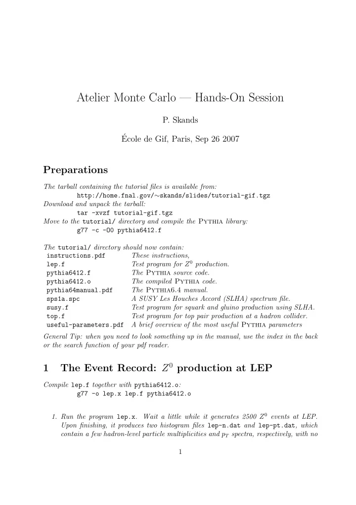
Atelier Monte Carlo — Hands-On Session P. Skands ´ Ecole de Gif, Paris, Sep 26 2007 Preparations The tarball containing the tutorial files is available from: http://home.fnal.gov/ ∼ skands/slides/tutorial-gif.tgz Download and unpack the tarball: tar -xvzf tutorial-gif.tgz Move to the tutorial/ directory and compile the Pythia library: g77 -c -O0 pythia6412.f The tutorial/ directory should now contain: These instructions, instructions.pdf Test program for Z 0 production. lep.f The Pythia source code. pythia6412.f pythia6412.o The compiled Pythia code. The Pythia6.4 manual. pythia64manual.pdf A SUSY Les Houches Accord (SLHA) spectrum file. sps1a.spc Test program for squark and gluino production using SLHA. susy.f Test program for top pair production at a hadron collider. top.f useful-parameters.pdf A brief overview of the most useful Pythia parameters General Tip: when you need to look something up in the manual, use the index in the back or the search function of your pdf reader. The Event Record: Z 0 production at LEP 1 Compile lep.f together with pythia6412.o : g77 -o lep.x lep.f pythia6412.o 1. Run the program lep.x . Wait a little while it generates 2500 Z 0 events at LEP. Upon finishing, it produces two histogram files lep-n.dat and lep-pt.dat , which contain a few hadron-level particle multiplicities and p T spectra, respectively, with no 1
cuts applied. Start by just looking at these distributions. Start gnuplot and plot the distribution of the number of tracks at LEP by: plot "lep-n.dat" using 1:2 with histeps Q: Why are only the bins with an even number of tracks populated? Now plot the p T spectrum of charged particles at LEP by: plot "lep-pt.dat" using 1:2 with histeps The remaining columns contain the same data for charged pions, charged kaons, pro- tons, and photons, respectively. Q: Who has the hardest p T spectrum: pions, kaons, or protons? 2. Run the program lep.x again and study the event records which are printed out (tip: a parenthesis (rho+) around a particle means it has decayed), in particular the correspondence between particle names and PDG codes ( K(I,2) ). Identify the PDG codes for: pions, kaons, protons, photons, gluons, and the quarks. (tip: the PDG codes and the event record are described in the Pythia manual, Chapter 5.) 3. Q: how do the multiplicities change if you switch off final-state radiation? Open lep.f in an editor and add a bit of code towards the top of the program: CALL PYGIVE(’MSTP(71)=0’) Recompile and run lep.x . 4. Finally, see how things change at ILC. Open lep.f again and change the center-of- mass energy, ECM , to 500 GeV. Again make a note of how the average track multi- plicities change. Remember to switch final-state radiation back on. Q: what changes if you switch off “electron ISR” ( MSTP(11)=0 )? (hint: radiative return.) 2 Tops at the Tevatron and LHC 1. The program top.f is just a copy of lep.f with small changes so that it now produces top pairs at Run II of the Tevatron. The multiplicity histograms have also been made twice as wide to accommodate the increased number of final-state particles. Compile the executable using: g77 -o top.x top.f pythia6412.o It produces the files top-n.dat and top-pt.dat , just like the ones before. The first thing you will notice is that the event records printed out at the beginning are signif- icantly longer, and that it now takes more time to generate events. If your computer is slow, change top.f so that, e.g., only 1000 events are generated. 2. Compare the average multiplicities and p ⊥ spectra with those you got at LEP. 3. Q: How do things change if you switch off: ISR ( MSTP(61)=0 ), FSR ( MSTP(71)=0 ), or the Underlying Event ( MSTP(81)=0 )? 2
4. Change the program so that it generates top pairs at LHC instead. Note: you need to change the CM energy, the beam types (in CALL PYINIT ), and possibly again the size of the multiplicity histograms (don’t use more than 100 bins, Pythia ’s internal package is limited to at most 100 bins). Congratulations! Event generation just got really, really slow... but then, you are now producing several hundred hadrons per collision, including decays and all the other stuff I mentioned yesterday. Q: the multiplicities change a lot. Do the p T spectra change? 3 The SUSY Les Houches Accord — gluinos, squarks, and jets 1. The third test program susy.f contains the commands for reading in a SUSY Les Houches Accord spectrum, here for the so-called SPS1a parameter point. Open the file sps1a.spc and familiarize yourself with what information is written there, and with the format (tip: you can check out the SUSY Les Houches Accord paper, hep- ph/0311123). 2. The program generates stop pairs at the LHC. It now only plots the charged particle multiplicity but then also uses a primitive jet finder internal to Pythia , a simple so-called UA1 cone algorithm. You shouldn’t use it for serious studies, but it is good enough here. (tip: look up PYCELL in the manual to find out what it does.) The jet numbers are in the file susy-njets.dat ; the first column is the x axis as usual, and the three data columns are n 100 , n 50 , and n 25 , respectively, where the subscript denotes the jet energy in GeV. The file susy-etjets.dat contain the E T spectra of jets, with the data columns representing jets 1 through 6. Q: compare the charged particle multiplicity in these events with what you had for top. Are they more or less busy? Also take a look at the jet numbers and p T spectra, just to make sure you understand what’s in the various columns and how to plot them (as provided, they are unnormalized, for instance). 3. Now try switching off initial-state radiation using MSTP(61) as above. Q: what changes? 4. Switch off the underlying event using MSTP(81) like above. Which jet distribution changes most? 4 Interface to ALPGEN 1. Download the Alpgen code from the web: http://mlm.home.cern.ch/mlm/alpgen/ This tarball does not create its own directory, so unpack it in a directory you create, then do a make in that directory. 3
2. Now you are ready to use Alpgen . In this exercise, you will use it to study W + 2 jets. Go to the wjetwork directory. Do a make gen in there to prepare the necessary executables. 3. Open the input file and familiarize yourself with its contents. The first keyword is mode . It should be 1 for the initial generation run ( → weighted events) and 2 for the subsequent unweighting run ( → unweighted events). Also familiarize yourself with the keyword controlling the “grid” setting. You should probably consult the Alpgen manual if you are unsure what it means (or if you are curious what any of the other keywords mean). Two additional keywords you will need further down in this exercise are: ebeam 7000 and ih2 1 , which will change the default Alpgen settings (= Tevatron) to the beam type and energy relevant for the LHC. 4. Now you are ready to start generating events. Run ./wjetgen < input This will generate events of the kind and number specified in input . 5. Now make an unweighted sample. Do this by changing the mode keyword in input to 2. Run ./wjetgen < input again. This last step produced two files we will need for the interface to Pythia : the first is w2j.unw . This file actually contains the events, one by one, in Alpgen ’s own format. The second is w2j unw.par , which contains “global” information, like the beam type used, the parton distributions used, the cross section, etc. 6. Alpgen provides ready-made routines for interfacing to Pythia . From the Alpgen root go to the pylib directory and do a make there. This will compile the program pyuser , which will read the files you just produced and pass them to Pythia for show- ering and hadronization. Copy the two w2j files to this directory and run pyuser , just to see what it does. 7. Now open pyuser and familiarize yourself with it. Don’t worry about all the stuff which is commented out. Concentrate on what the code actually does. You will see many similarities to what we were doing earlier. First, there is an initialization call to PYINIT , with the special keyword USER , which tells Pythia that we will be inputting external events. Then, there is an event loop with calls to PYEVNT , just like before. You can now put your event-by-event analysis, jet clustering, cuts, etc, after the calls to PYEVNT , just like before. Q: try to adapt some of the things from the earlier programs to run in this code, e.g. make a histogram of the charged multiplicity. 8. Now you are ready to use Alpgen – Pythia for more serious studies. Go ahead, and fun will come. 4
Recommend
More recommend
Explore More Topics
Stay informed with curated content and fresh updates.

