Asset Pricing Chapter VI. Risk Aversion and Investment Decisions, - PowerPoint PPT Presentation
6.1 Introduction 6.2 More About Utility Functions 6.3 Opportunity Set in the Mean-Variance Space 6.4 The Optimal Portfolio: A Separation Theorem 6.5 Conclusions Asset Pricing Chapter VI. Risk Aversion and Investment Decisions, Part II: Modern
6.1 Introduction 6.2 More About Utility Functions 6.3 Opportunity Set in the Mean-Variance Space 6.4 The Optimal Portfolio: A Separation Theorem 6.5 Conclusions Asset Pricing Chapter VI. Risk Aversion and Investment Decisions, Part II: Modern Portfolio Theory June 20, 2006 Asset Pricing
6.1 Introduction 6.2 More About Utility Functions 6.3 Opportunity Set in the Mean-Variance Space 6.4 The Optimal Portfolio: A Separation Theorem 6.5 Conclusions � N i = 1 a i (˜ { a 1 , a 2 ,..., a N } EU ( Y 0 ( 1 + r f ) + r i − r f )) max � N i = 1 w i Y 0 (˜ = { w 1 , w 2 ,..., w N } EU ( Y 0 ( 1 + r f ) + r i − r f )) max (1) X N n h io n o ˜ max EU Y 0 ( 1 + r f ) + i = 1 w i (˜ r i − r f ) = EU { Y 0 [ 1 + ˜ r P ] } = EU Y 1 (2) { w 1 , w 2 ,..., wN } Asset Pricing
6.1 Introduction 6.2 More About Utility Functions 6.3 Opportunity Set in the Mean-Variance Space Backward Induction 6.4 The Optimal Portfolio: A Separation Theorem 6.5 Conclusions More About Utility Functions Step 1: The consumption-savings decision C 0 + S 0 = Y 0 Step 2: The Portfolio Problem N risky assets with ( 1 − � N i = 1 w i )( Y 0 − C 0 ) ( w 1 ( Y 0 − C 0 ) , w 2 ( Y 0 − C 0 ) , .., w N ( Y 0 − C 0 )) Step 3: Tomorrow’s Consumption Choice U ( c 1 , c 2 , ..... c n ) p 1 θ c 1 θ + .. + p m θ c m θ ≤ Y θ . � � � N Y θ = ( Y 0 − C 0 ) ( 1 + r f ) + i = 1 w i ( r i θ − r f ) Asset Pricing
6.1 Introduction 6.2 More About Utility Functions 6.3 Opportunity Set in the Mean-Variance Space Backward Induction 6.4 The Optimal Portfolio: A Separation Theorem 6.5 Conclusions Backward Induction U ( Y θ ) ≡ def ( c 1 θ ,..., c m θ ) u ( c 1 θ , ..., c m θ ) max s.t. p 1 θ c 1 θ + .. + p m θ c m θ ≤ Y θ . � EU ( ˜ max Y ) = π θ U ( Y θ ) . { w 1 , w 2 , ... w N } θ Asset Pricing
6.1 Introduction 6.2 More About Utility Functions 6.3 Opportunity Set in the Mean-Variance Space Backward Induction 6.4 The Optimal Portfolio: A Separation Theorem 6.5 Conclusions From Utility on wealth to utility on return: max EU ( ˜ r P )) = def max E ˆ Y ) = max EU (( Y 0 − C 0 )( 1 + ˜ U (˜ r P ) "Mean-Variance Utility Function" Asset Pricing
6.1 Introduction 6.2 More About Utility Functions 6.3 Opportunity Set in the Mean-Variance Space Backward Induction 6.4 The Optimal Portfolio: A Separation Theorem 6.5 Conclusions Taylor series approximation: � � � � �� + U ′ � � �� � � �� ˜ ˜ ˜ ˜ ˜ EU Y = U E Y E Y Y − E Y 2 U ′′ � � �� � � �� 2 + 1 ˜ ˜ ˜ E Y Y − E Y + H 3 (3) Computing expected utility using this approximation: � � �� + U ′ � � �� � � �� EU ( ˜ ˜ ˜ E ( ˜ ˜ Y ) = U E Y E Y Y ) − E Y � �� � = 0 + 1 2 U ′′ � � �� � � �� 2 ˜ ˜ ˜ E Y E Y − E Y + EH 3 � �� � = σ 2 (˜ w ) � � �� + 1 2 U ′′ � � �� σ 2 � � ˜ ˜ ˜ = + EH 3 U E Y E Y Y Asset Pricing
Two perfect correlated risky assets 6.1 Introduction Two imperfectly correlated risky assets 6.2 More About Utility Functions Two perfectly negative correlated risky assets 6.3 Opportunity Set in the Mean-Variance Space One Risky and One Risk Free Asset 6.4 The Optimal Portfolio: A Separation Theorem One Risk Free Asset and "N" Risky Assets 6.5 Conclusions Portfolio optimization problem Description of the Opportunity Set in the Mean-Variance Space: The Gains form Diversification and the Efficient Frontier " The main idea of this section is the following: The expected return to a portfolio is the weighted average of the expected returns of the assets composing the portfolio. The same result is not generally true for the variance: the variance of a portfolio is generally smaller than the weighted average of the variances of individual asset returns corresponding to this portfolio . Therein lies the gain from diversification". Asset Pricing
Two perfect correlated risky assets 6.1 Introduction Two imperfectly correlated risky assets 6.2 More About Utility Functions Two perfectly negative correlated risky assets 6.3 Opportunity Set in the Mean-Variance Space One Risky and One Risk Free Asset 6.4 The Optimal Portfolio: A Separation Theorem One Risk Free Asset and "N" Risky Assets 6.5 Conclusions Portfolio optimization problem The typical investor likes expected return µ R and dislikes standard deviation σ R Recall that an asset (or portfolio) A is said to mean-variance dominate an asset (or portfolio B) if µ A ≥ µ B while σ A ≥ σ B Define the efficient frontier as the locus of all non-dominated portfolios in the mean-standard deviation space. By definition, no ("rational") mean-variance investor would choose to hold a portfolio not located on the efficient frontier. Asset Pricing
Two perfect correlated risky assets 6.1 Introduction Two imperfectly correlated risky assets 6.2 More About Utility Functions Two perfectly negative correlated risky assets 6.3 Opportunity Set in the Mean-Variance Space One Risky and One Risk Free Asset 6.4 The Optimal Portfolio: A Separation Theorem One Risk Free Asset and "N" Risky Assets 6.5 Conclusions Portfolio optimization problem The Efficient Frontier: Two perfect correlated risky assets σ R = w 1 σ 1 + ( 1 − w 1 ) σ 2 . r 1 + ¯ r 2 − ¯ r 1 µ R = ¯ ( σ R − σ 1 ) , σ 2 − σ 1 m –� r 2 m R –� r 1 s 1 s R s 2 s Asset Pricing
Two perfect correlated risky assets 6.1 Introduction Two imperfectly correlated risky assets 6.2 More About Utility Functions Two perfectly negative correlated risky assets 6.3 Opportunity Set in the Mean-Variance Space One Risky and One Risk Free Asset 6.4 The Optimal Portfolio: A Separation Theorem One Risk Free Asset and "N" Risky Assets 6.5 Conclusions Portfolio optimization problem The Efficient Frontier: Two imperfectly correlated risky assets m R B D C A s R Asset Pricing
Two perfect correlated risky assets 6.1 Introduction Two imperfectly correlated risky assets 6.2 More About Utility Functions Two perfectly negative correlated risky assets 6.3 Opportunity Set in the Mean-Variance Space One Risky and One Risk Free Asset 6.4 The Optimal Portfolio: A Separation Theorem One Risk Free Asset and "N" Risky Assets 6.5 Conclusions Portfolio optimization problem The Efficient Frontier: Two perfectly negative correlated risky assets m –� r 2 –� –� r 1 – r 2 s 2 s 1 s 2 s 1 –� –� + –� s 1 + s 2 –� –� r 1 r 2 + s R r 1 r 2 s 1 + s 2 s 1 + s 2 s 1 + s 2 s 1 + s 2 –� r 1 s 1 s 2 s –� –� r 1 – r 2 s 2 s 1 –� –� + + s 1 + s 2 r 1 r 2 s R s 1 + s 2 s 1 + s 2 Asset Pricing
Two perfect correlated risky assets 6.1 Introduction Two imperfectly correlated risky assets 6.2 More About Utility Functions Two perfectly negative correlated risky assets 6.3 Opportunity Set in the Mean-Variance Space One Risky and One Risk Free Asset 6.4 The Optimal Portfolio: A Separation Theorem One Risk Free Asset and "N" Risky Assets 6.5 Conclusions Portfolio optimization problem One Risky and One Risk Free Asset m –� r 2 –� r 1 s 2 s –� –� r 2 – r 1 s 2 Asset Pricing
Two perfect correlated risky assets 6.1 Introduction Two imperfectly correlated risky assets 6.2 More About Utility Functions Two perfectly negative correlated risky assets 6.3 Opportunity Set in the Mean-Variance Space One Risky and One Risk Free Asset 6.4 The Optimal Portfolio: A Separation Theorem One Risk Free Asset and "N" Risky Assets 6.5 Conclusions Portfolio optimization problem One Risk Free Asset and "N" Risky Assets m T F E r f s Asset Pricing
Two perfect correlated risky assets 6.1 Introduction Two imperfectly correlated risky assets 6.2 More About Utility Functions Two perfectly negative correlated risky assets 6.3 Opportunity Set in the Mean-Variance Space One Risky and One Risk Free Asset 6.4 The Optimal Portfolio: A Separation Theorem One Risk Free Asset and "N" Risky Assets 6.5 Conclusions Portfolio optimization problem The portfolio optimization problem: � � min w i w j σ ij w i ′ s i j s . t . � w i ¯ r i = µ ( QP ) i � w i = 1 i Asset Pricing
6.1 Introduction 6.2 More About Utility Functions 6.3 Opportunity Set in the Mean-Variance Space 6.4 The Optimal Portfolio: A Separation Theorem 6.5 Conclusions A Separation Theorem The Optimal Portfolios of Two Differently Risk Aversion Investors m Agent 2 Agent 1 T r f s Asset Pricing
6.1 Introduction 6.2 More About Utility Functions 6.3 Opportunity Set in the Mean-Variance Space 6.4 The Optimal Portfolio: A Separation Theorem 6.5 Conclusions 6.5 Conclusions MPT: A normative interpretation Spelling out the information requirements for portfolio analysis Using historical returns for asset allocation purposes Static vs. Dynamic portfolio allocation Asset Pricing
6.1 Introduction 6.2 More About Utility Functions 6.3 Opportunity Set in the Mean-Variance Space 6.4 The Optimal Portfolio: A Separation Theorem 6.5 Conclusions Key concepts Backward induction; indirect utility Gains from diversification Efficient Frontier Optimal Portfolio Two fund or separation theorem Asset Pricing
Recommend
More recommend
Explore More Topics
Stay informed with curated content and fresh updates.

