+ arXiv:1501.01715 + Richard Cleve & Rolando Somma Andrew - PowerPoint PPT Presentation
Hamiltonian simulation with nearly optimal dependence on all parameters Dominic Berry + arXiv:1501.01715 + Richard Cleve & Rolando Somma Andrew Childs & Robin Kothari Why is this important? Why is this important? Aharonov
Hamiltonian simulation with nearly optimal dependence on all parameters Dominic Berry + arXiv:1501.01715 + Richard Cleve & Rolando Somma Andrew Childs & Robin Kothari
Why is this important?
Why is this important? Aharonov & Ta-Shma 2003: Algorithm to simulate sparse Hamiltonians Childs, Cleve, Jordan, Yonge-Mallo Harrow, Hassidim, Lloyd 2009: Quantum algorithm for 2009: Quantum algorithm to NAND trees solve linear systems Clader, Jacobs, Sprouse Berry Wang 2013: Quantum algorithm for 2014: Quantum algorithm 2014: Quantum algorithm for scattering problems for differential equations effective electrical resistance
The simulation problem Problem: Given a Hamiltonian 𝐼 , simulate 𝑒 𝑒𝑢′ 𝜔(𝑢′) = −𝑗𝐼 𝜔(𝑢′) for time 𝑢 and error no more than 𝜁 . Inputs: 𝐼 , 𝑢 , 𝜁 Parameters of 𝐼 : 𝑒 – sparseness 𝑂 – dimension 𝐼 or 𝐼 max – norms of the Hamiltonian
Progression of results Standard method: Product formula 𝑃(𝑒 4 𝐼 𝑢 1+𝜀 /𝜗 𝜀 ) Advanced methods: Compressed product formula Quantum walks or Taylor series 𝑃(𝑒 𝐼 max 𝑢/ 𝜗) 𝑃(𝑒 2 𝐼 max 𝑢 × polylog) New method: Combined approach 𝑃(𝑒 𝐼 max 𝑢 × polylog)
Main results 𝑃 𝑒 𝐼 max 𝑢 × polylog Complexity: Near-linear in 𝑒 , like quantum walk approach. Polylogarithmic in 𝜁 , like compressed product formulae. What is the polylog factor? log(𝜐/𝜁) Queries: polylog ≡ log log(𝜐/𝜁) log 2 (𝜐/𝜁) Gates: polylog ≡ log log(𝜐/𝜁) 𝜐 = 𝑒 𝐼 max 𝑢 Ω 𝑒 𝐼 max 𝑢 + polylog Lower bound:
Model Sparse Hamiltonians Query: An efficient algorithm to determine the positions and values of non-zero entries.
Standard method Use decomposition as 𝑁 𝐼 = 𝐼 𝑙 𝑙=1 Divide time into 𝑠 intervals and use product formula: 𝑠 𝑁 𝑓 −𝑗𝐼𝑢 ≈ 𝑓 −𝑗𝐼 𝑙 𝑢/𝑠 𝑙=1 S. Lloyd, Science 273 , 1073 (1996).
Advanced methods Compressed product formulae 1. Implementing Taylor series 2. Quantum walks 3. Superposition of quantum walk steps 4. D. W. Berry, A. M. Childs, R. Cleve, R. Kothari, R. D. Somma , STOC ‘14; arXiv:1312.1414 (2013). D. W. Berry, A. M. Childs, R. Cleve, R. Kothari, R. D. Somma, arXiv:1412.4687 (2014). D. W. Berry, A. M. Childs, Quantum Information and Computation 12 , 29 (2012). D. W. Berry, A. M. Childs, R. Kothari, arXiv:1501.01715 (2015).
Compressed product formulae Crucial ideas we use in new work: Break evolution into segments. 1. In each segment use controlled operations. 2. Apply oblivious amplitude amplification to achieve 3. result deterministically.
Break into segments |𝜔〉 |𝜔′〉 𝑓 −𝑗𝐼𝑢/𝑠 . . . . . . . . . . . . . 1 2 3 5 6 7 4 10 9 t 0 1 2 4 4 4 4 4 4 4
Evolution using control qubits 𝑉 is self-inverse 〈0| 0 𝑆 𝑄 𝑆 𝑓 −𝑗𝑉𝑢 |𝜔〉 |𝜔〉 𝑉 R. Cleve, D. Gottesman, M. Mosca, R. Somma, D. Yonge-Mallo, STOC ‘09; arXiv:0811.4428 (2008).
Oblivious amplitude amplification measure |𝑑 0 𝑛 〉 𝑋 † 𝑋 |𝜔′〉 |𝜔〉 𝑉 𝑉 𝑉 𝑘 𝑘 𝑘 . . . . . . . . . . . . . 1 2 3 5 6 7 4 10 9 t 0 1 2 4 4 4 4 4 4 4
Oblivious amplitude amplification |𝑑 0 𝑛 〉 𝑋 † 𝑋 |𝜔′〉 |𝜔〉 𝑉 𝑉 𝑉 𝑘 𝑘 𝑘 . . . . . . . . . . . . . 1 2 3 5 6 7 4 10 9 t 0 1 2 4 4 4 4 4 4 4
Oblivious amplitude amplification 𝑋 † 𝑋 success! |𝜔′〉 |𝜔〉 𝑉 𝑉 𝑉 𝑘 𝑘 𝑘 . . . . . . . . . . . . . 1 2 3 5 6 7 4 10 9 t 0 1 2 4 4 4 4 4 4 4
Advanced methods Compressed product formulae 1. Implementing Taylor series 2. Quantum walks 3. Superposition of quantum walk steps 4. D. W. Berry, A. M. Childs, R. Cleve, R. Kothari, R. D. Somma , STOC ‘14; arXiv:1312.1414 (2013). D. W. Berry, A. M. Childs, R. Cleve, R. Kothari, R. D. Somma, arXiv:1412.4687 (2014). D. W. Berry, A. M. Childs, Quantum Information and Computation 12 , 29 (2012). D. W. Berry, A. M. Childs, R. Kothari, arXiv:1501.01715 (2015).
Implementing Taylor series Break Hamiltonian evolution into 𝑠 segments and use 𝐿 𝑓 −𝑗𝐼𝑢/𝑠 ≈ 1 𝑙! −𝑗𝐼𝑢/𝑠 𝑙 𝑙=0 Aim to perform using controlled operations. 𝑙 〈0| 0 𝑋 † 𝑋 𝑓 −𝑗𝐼𝑢/𝑠 |𝜔〉 |𝜔〉 𝐼 𝑙
Implementing Taylor series Expand 𝐼 as sum of unitaries 𝑁 𝐼 ≈ 𝛿 𝑉 ℓ ℓ=1 Exponential is then 𝐿 𝑁 𝑁 𝑁 𝑓 −𝑗𝐼𝑢/𝑠 ≈ ⋯ −𝑗𝑢/𝑠 𝑙 𝑉 ℓ 1 𝑉 ℓ 2 ⋯ 𝑉 ℓ 𝑙 𝑙! 𝑙=0 ℓ 1 =1 ℓ 2 =1 ℓ 𝑙 =1 𝑙 ℓ 1 measure |0〉 𝑋 † 𝑋 ℓ 2 ℓ 𝐿 𝑓 −𝑗𝐼𝑢/𝑠 |𝜔〉 |𝜔〉 𝑉 ℓ 1 𝑉 ℓ 2 𝑉 ℓ 𝐿
Advanced methods Compressed product formulae 1. Implementing Taylor series 2. Quantum walks 3. Superposition of quantum walk steps 4. D. W. Berry, A. M. Childs, R. Cleve, R. Kothari, R. D. Somma , STOC ‘14; arXiv:1312.1414 (2013). D. W. Berry, A. M. Childs, R. Cleve, R. Kothari, R. D. Somma, arXiv:1412.4687 (2014). D. W. Berry, A. M. Childs, Quantum Information and Computation 12 , 29 (2012). D. W. Berry, A. M. Childs, R. Kothari, arXiv:1501.01715 (2015).
Quantum walks Classical walk Position is integer 𝑦 . Step is map 𝑦 → 𝑦 ± 1 with equal probability. Standard quantum walk Quantum position and coin registers |𝑦, 𝑑〉 . Alternates coin and step operators, 𝐷 𝑦, ±1 = 𝑦, −1 ± 𝑦, 1 / 2 𝑇 𝑦, 𝑑 = |𝑦 + 𝑑, 𝑑〉 Szegedy quantum walk Two subsystems with arbitrary dimension. Step is controlled reflection.
Szegedy quantum walk Controlled reflections: 𝑘 〈𝑘| ⊗ (2|𝑑 𝑘 〉〈𝑑 𝑘 | − 𝕁) 𝑘 reflect about |𝑑 𝑘 〉 controlled on 𝑘 |𝑑 𝑘 〉 After doing this we swap the two systems. Step operation is 𝑉 = 𝑗 × SWAP × controlled reflection Controlled reflection can be achieved with controlled preparation: 𝑈 = 𝑘 〈𝑘| ⊗ |𝑑 𝑘 〉 𝑘 M. Szegedy, FOCS ‘04; arXiv:quant-ph/0401053 (2004).
Szegedy walk for Hamiltonians Three part process: Start with state in one of the subsystems, and perform 1. controlled state preparation 𝑈 . 𝑈 Perform steps of quantum walk 𝑉 to approximate 2. Hamiltonian evolution. 𝑉 Invert controlled state preparation, so final state is in one of 3. the subsystems. Each 𝑉 or 𝑈 uses 𝑈 † 𝑃(1) calls to 𝐼 . A. M. Childs, Commun. Math. Phys. 294 , 581 (2009).
Eigenvalues of walk Hamiltonian 𝐼 has eigenvalues 𝜇 . Step 𝑉 has eigenvalues 𝜈 ± = ±𝑓 ±𝑗 arcsin 𝜇 Evolution under the Hamiltonian has eigenvalues 𝜌 − arcsin 𝜇 arcsin 𝜇 𝑓 −𝑗𝜇𝑢 𝜇 |𝜈 − 〉 |𝜈 + 〉 Given knowledge of + or − we can correct to 𝑉 𝑑 with eigenvalues 𝜈 = 𝑓 −𝑗 arcsin 𝜇
Eigenvalues of walk Step 𝑉 𝑑 has eigenvalues 𝜈 = 𝑓 −𝑗 arcsin 𝜇 We aim for 𝑓 −𝑗𝜇𝑢 Try superposition of operations 𝐿 𝑙 𝑉 sup = 𝛽 𝑙 𝑉 𝑑 𝜌 − arcsin 𝜇 arcsin 𝜇 𝑙=−𝐿 𝜇 |𝜈 − 〉 |𝜈 + 〉 0 〈0| 𝑋 𝑋 † |𝜔〉 𝑉 sup |𝜔〉 𝑙 𝑉 𝑑
Choosing values for 𝛽 𝑙 We aim to find 𝛽 𝑙 such that 𝐿 𝛽 𝑙 𝜈 𝑙 ≈ 𝑓 −𝑗𝜇𝑢 𝑙=−𝐿 The formula for 𝜈 gives 𝑓 −𝑗𝜇𝑢 = exp 𝑢 2 𝜈 − 1 𝜈 But this is the generating function for Bessel functions! ∞ = exp 𝑢 2 𝜈 − 1 𝐾 𝑙 𝑢 𝜈 𝑙 𝜈 𝑙=−∞ We can choose 𝛽 𝑙 just from Bessel functions.
Without correcting the step We aim to find 𝛽 𝑙 such that 𝐿 𝑙 ≈ 𝑓 −𝑗𝜇𝑢 𝛽 𝑙 𝜈 ± 𝑙=−𝐿 The formula for 𝜈 ± gives 𝑓 −𝑗𝜇𝑢 = exp − 𝑢 2 𝜈 ± − 1 𝜈 ± But this is the generating function for Bessel functions! ∞ = exp − 𝑢 2 𝜈 ± − 1 𝑙 𝐾 𝑙 −𝑢 𝜈 ± 𝜈 ± 𝑙=−∞ We can choose 𝛽 𝑙 just from Bessel functions. We don’t need to distinguish + from − or correct the step!
The complete algorithm Map into doubled Hilbert space. Divide the time into 𝑠 = 𝑒 𝐼 max 𝑢 segments. 0 t For each segment: 1. Perform the superposition. Use amplitude amplification to 2. obtain success deterministically. 0 〈0| 𝑋 𝑋 † 𝐾 𝑙 (𝑦) |𝜔〉 𝑉 sup |𝜔〉 𝑉 𝑙 Map back to original Hilbert space. Total complexity: 𝑒 𝐼 max 𝑢 × 𝐿
Choosing the value of 𝐿 Bessel function may be bounded as 𝐾 𝑙 𝑦 ≤ 1 𝑦 𝑙 𝑙! 2 Scaling is the same as for Taylor series! 𝐾 𝑙 (1) We can choose 𝐿 to be polylog log(𝜐/𝜁) 𝐿 ∼ log log(𝜐/𝜁) Overall scaling is 𝑃(𝑒 𝐼 max 𝑢 × polylog) 𝑙
Single-segment approach 𝐾 𝑙 (𝑒 𝐼 max 𝑢) polylog 𝑙 𝑒 𝐼 max 𝑢 Choosing segment sizes 𝜐 𝛽 gives complexity 𝜐 1+𝛽/2 + 𝜐 1−𝛽/2 log(1/𝜁)
Recommend
More recommend
Explore More Topics
Stay informed with curated content and fresh updates.
