Artificial Neural Networks (Part 2) Gradient Descent Learning and - PDF document

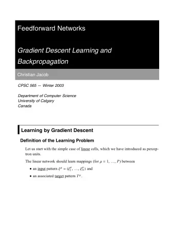
Artificial Neural Networks (Part 2) Gradient Descent Learning and Backpropagation Christian Jacob CPSC 533 — Winter 2001 Learning by Gradient Descent Definition of the Learning Problem Let us start with the simple case of linear cells, which we have introduced as percep - tron units. The linear network should learn mappings (for m = 1, …, P ) between m L and Ë an input pattern x m = H x 1 m , …, x N Ë an associated target pattern T m .

2 05.2-Backprop-Printout.nb Figure 1. Perceptron m of cell i for the input pattern x m is calculated as The output O i m = ‚ H w ki ÿ x k m L O i (1) k m for input pat - The goal of the learning procedure is, that eventually the output O i m : tern x m corresponds to the desired output T i ! T i m = ‚ m = H w ki ÿ x k m L O i (2) k Explicit Solution (Linear Network) For a linear network, the weights that satisfy Equation (2) can be calculated explic - itly using the pseudo-inverse: w ik = 1 - 1 L ml x k m H Q k P ‚ l T i ÅÅÅÅ (3) ml

05.2-Backprop-Printout.nb 3 Q ml = 1 m x k P ‚ l ÅÅÅÅ x k (4) k ‡ Correlation Matrix Here Q ml is a component of the correlation matrix Q k of the input patterns: 1 x k 1 1 x k 2 1 x k P i y … x k x k x k j z j z j z j z Q k = . . . . j z (5) j z j z j z P x k 1 P x k P … … k { x k x k You can check that this is indeed a solution by verifying m = T i m . ‚ w ik x k (6) k ‡ Caveat Note that Q - 1 only exists for linearly independent input patterns. That means, if there are a i such that for all k = 1, …, N 1 + a 2 x k 2 + … + a P x k P = 0, a 1 x k (7) m cannot be selected independently from each other, and the then the outputs O i problem is NOT solvable. Learning by Gradient Descent (Linear Network) Let us now try to find a learning rule for a linear network with M output units. ÷÷ ” Starting from a random initial weight setting w 0 , the learning procedure should find a solution weight matrix for Equation (2). ‡ Error Function ÷÷ L : ” For this purpose, we define a cost or error function E H w

4 05.2-Backprop-Printout.nb M P ”L = 1 m L 2 m - O m E H w H T m 2 ‚ ‚ ÅÅÅÅ m = 1 m= 1 (8) M P 2 i y ”L = 1 j z j z E H w m - ‚ H w km ÿ x k m L 2 „ „ j j T m z ÅÅÅÅ z k { k m = 1 m= 1 ÷÷ L ¥ 0 will approach zero as w ” ÷÷ = 8 w km < satisfies Equation (2). ” E H w This cost function is a quadratic function in weight space. ‡ Paraboloid ÷÷ L is a paraboloid with a single global minimum. ” Therefore, E H w << RealTime3D` Plot3D @ x 2 + y 2 , 8 x, - 5, 5 < , 8 y, - 5, 5 <D ;

05.2-Backprop-Printout.nb 5 ContourPlot @ x 2 + y 2 , 8 x, - 5, 5 < , 8 y, - 5, 5 <D ; 4 2 0 -2 -4 -4 -2 0 2 4 If the pattern vectors are linearly independent—i.e., a solution for Equation (2) exists—the minimum is at E = 0. ‡ Finding the Minimum: Following the Gradient ÷÷ L in weight space by following the negative ” We can find the minimum of E H w gradient ÷ L ” ÷ L = -∑ E H w ” E H w ÷ ” (9) ” -∑ w ÅÅÅÅÅÅÅÅÅÅÅÅÅÅÅÅ ÅÅÅ ∑ w We can implement this gradient strategy as follows: ‡ Changing a Weight ÷÷ is changed by D w ki proportionate to the E gradient at the ” Each weight w ki œ w current weight position (i.e., the current settings of all the weights):

6 05.2-Backprop-Printout.nb ”L D w ki = -h ∑ E H w (10) ÅÅÅÅÅÅÅÅÅÅÅÅÅÅÅÅÅ Å ∑ w ki ‡ Steps Towards the Solution i M P 2 y j z i y j z j z j 1 z ∑ j z j z m - ‚ H w nm ÿ x n m L D w ki = -h j T m j z j 2 „ „ z ÅÅÅÅÅÅÅÅÅÅÅÅ Å ÅÅÅÅ z j z j z ∑ w ki j z k { n k { m = 1 m= 1 P M i 2 y j z i y j z D w ki = -h 1 j z j z ∑ j z m - ‚ j H w nm ÿ x n m L z j z 2 „ j„ j T m (11) j z ÅÅÅÅ ÅÅÅÅÅÅÅÅÅÅÅÅ Å z j z ∑ w ki z k { n k { m= 1 m = 1 P i y D w ki = -h 1 j z j z m - ‚ H w ni ÿ x n m L z H -x k m L j z 2 „ 2 j T i ÅÅÅÅ k { n m= 1 ‡ Weight Adaptation Rule P m - O i H T i m L x k m D w ki = h ‚ (12) m= 1 The parameter h is usually referred to as the learning rate . In this formula, the adaptation of the weights are accumulated over all patterns. ‡ Delta, LMS Learning If we change the weights after each presentation of an input pattern to the network, we get a simpler form for the weight update term: m - O i m L x k m D w ki = h H T i (13) or m x k m D w ki = h d i (14) with m = T i m - O i m . (15) d i

05.2-Backprop-Printout.nb 7 This learning rule has several names: Ë Delta rule Ë Adaline rule Ë Widrow-Hoff rule Ë LMS (least mean square) rule. Gradient Descent Learning with Nonlinear Cells We will now extend the gradient descent technique for the case of nonlinear cells, that is, where the activation/output function is a general nonlinear function g(x). † The input function is denoted by h H x L . † The output function g H h H x LL is assumed to be differentiable in x . ‡ Rewriting the Error Function The definition of the error function (Equation (8)) can be simply rewritten as follows: M P ”L = 1 m L 2 m - O m E H w H T m 2 ‚ ‚ ÅÅÅÅ m = 1 m= 1 (16) M P 2 i i y y ”L = 1 j j z z j j z z m - g m L E H w j‚ H w km ÿ x k 2 „ „ j T m j j z z ÅÅÅÅ z z k k { { k m = 1 m= 1 ‡ Weight Gradients Consequently, we can compute the w ki gradients: ”L P ∑ E H w m - g H h i = ‚ H T i m LL ÿ g £ H h i m L ÿ x k m (17) ÅÅÅÅÅÅÅÅÅÅÅÅÅÅÅÅÅÅ ∑ w ki m= 1

8 05.2-Backprop-Printout.nb ‡ From Weight Gradients to the Learning Rule This eventually (after some more calculations) shows us that the adaptation term D w ki for w ki has the same form as in Equations (10), (13), and (14), namely: m x k m D w ki = h d i (18) where m = H T i m - O i m L ÿ g £ H h i m L (19) d i Suitable Activation Functions The calculation of the above d terms is easy for the following functions g , which are commonly used as activation functions: ‡ Hyperbolic Tangens: g H x L = tanh b x (20) g £ H x L = b H 1 - g 2 H x LL Hyperbolic Tangens Plot: Plot @ Tanh @ x D , 8 x, - 5, 5 <D ; 1 0.5 -4 -2 2 4 -0.5 -1

05.2-Backprop-Printout.nb 9 Plot of the first derivative: Plot @ Tanh' @ x D , 8 x, - 5, 5 <D ; 1 0.8 0.6 0.4 0.2 -4 -2 2 4 Check for equality with 1 - tanh 2 x Plot @ 1 - Tanh @ x D 2 , 8 x, - 5, 5 <D ; 1 0.8 0.6 0.4 0.2 -4 -2 2 4 Influence of the b parameter: p1 @ b _ D : = Plot @ Tanh @ b x D , 8 x, - 5, 5 < , PlotRange Ø All, DisplayFunction Ø Identity D p2 @ b _ D : = Plot @ Tanh' @ b x D , 8 x, - 5, 5 < , PlotRange Ø All, DisplayFunction Ø Identity D

10 05.2-Backprop-Printout.nb Table @ Show @ GraphicsArray @8 p1 @ b D , p2 @ b D<DD , 8 b , 1, 5 <D ; 1 1 0.8 0.5 0.6 -4 -2 2 4 0.4 -0.5 0.2 -4 -2 2 4 -1 1 1 0.8 0.5 0.6 -4 -2 2 4 0.4 -0.5 0.2 -4 -2 2 4 -1 1 1 0.8 0.5 0.6 -4 -2 2 4 0.4 -0.5 0.2 -4 -2 2 4 -1 1 1 0.8 0.5 0.6 -4 -2 2 4 0.4 -0.5 0.2 -4 -2 2 4 -1

05.2-Backprop-Printout.nb 11 1 1 0.8 0.5 0.6 -4 4 -2 2 0.4 -0.5 0.2 -4 -2 2 4 -1 Table @ Show @ GraphicsArray @8 p1 @ b D , p2 @ b D<DD , 8 b , 0.1, 1, 0.1 <D ; -4 -2 2 4 0.4 0.95 0.2 0.9 -4 -2 2 4 0.85 -0.2 -0.4 0.8 -4 -2 2 4 0.6 0.9 0.4 0.8 0.2 0.7 -4 -2 2 4 -0.2 0.6 -0.4 0.5 -0.6 -4 -2 2 4 0.75 0.5 0.8 0.25 0.6 -4 -2 2 4 -0.25 0.4 -0.5 -0.75 0.2 1 -4 -2 2 4 0.8 0.5 0.6 -4 -2 2 4 0.4 -0.5 0.2 -1

12 05.2-Backprop-Printout.nb 1 1 0.8 0.5 0.6 -4 -2 2 4 0.4 -0.5 0.2 -4 -2 2 4 -1 1 1 0.8 0.5 0.6 -4 4 -2 2 0.4 0.2 -0.5 -4 -2 2 4 -1 1 1 0.8 0.5 0.6 -4 4 -2 2 0.4 0.2 -0.5 -4 -2 2 4 -1 1 1 0.8 0.5 0.6 -4 -2 2 4 0.4 0.2 -0.5 -4 -2 2 4 -1 1 1 0.8 0.5 0.6 -4 -2 2 4 0.4 0.2 -0.5 -4 -2 2 4 -1

05.2-Backprop-Printout.nb 13 1 1 0.8 0.5 0.6 -4 -2 2 4 0.4 -0.5 0.2 -4 -2 2 4 -1 ‡ Sigmoid: 1 g H x L = ÅÅÅÅÅÅÅÅÅÅÅÅÅÅÅÅ ÅÅÅÅ Å 1 + e - 2 b x (21) g £ H x L = 2 b g H x L H 1 - g H x LL Sigmoid Plot: 1 sigmoid @ x_, b _ D : = ÅÅÅÅÅÅÅÅÅÅÅÅÅÅÅÅ ÅÅÅÅÅÅ 1 + E - 2 b x Plot @ sigmoid @ x, 1 D , 8 x, - 5, 5 <D ; 1 0.8 0.6 0.4 0.2 -4 -2 2 4 Plot of the first derivative:

14 05.2-Backprop-Printout.nb D @ sigmoid @ x, b D , x D 2 ‰ - 2 x b b ÅÅÅÅÅÅÅÅÅÅÅÅÅÅÅÅ ÅÅÅÅÅÅÅÅ ÅÅÅÅÅÅ H 1 + ‰ - 2 x b L 2 Plot @ D @ sigmoid @ x, 1 D , x D êê Evaluate, 8 x, - 5, 5 <D ; 0.5 0.4 0.3 0.2 0.1 -4 -2 2 4 Check for equality with 2 ÿ g ÿ H 1 - g L Plot @ 2 sigmoid @ x, 1 D H 1 - sigmoid @ x, 1 DL , 8 x, - 5, 5 <D ; 0.5 0.4 0.3 0.2 0.1 -4 -2 2 4 Influence of the b parameter:

05.2-Backprop-Printout.nb 15 p1 @ b _ D : = Plot @ sigmoid @ x, b D , 8 x, - 5, 5 < , PlotRange Ø All, DisplayFunction Ø Identity D p2 @ b _ D : = Plot @ D @ sigmoid @ x, b D , x D êê Evaluate, 8 x, - 5, 5 < , PlotRange Ø All, DisplayFunction Ø Identity D Table @ Show @ GraphicsArray @8 p1 @ b D , p2 @ b D<DD , 8 b , 1, 5 <D ; 1 0.5 0.8 0.4 0.6 0.3 0.4 0.2 0.2 0.1 -4 -2 2 4 -4 -2 2 4 1 1 0.8 0.8 0.6 0.6 0.4 0.4 0.2 0.2 -4 4 -4 4 -2 2 -2 2 1 1.4 1.2 0.8 1 0.6 0.8 0.6 0.4 0.4 0.2 0.2 -4 -2 2 4 -4 -2 2 4 1 2 0.8 1.5 0.6 1 0.4 0.5 0.2 -4 -2 2 4 -4 -2 2 4