ARTIFICIAL INTELLIGENCE Reinforcement learning Lecturer: Silja - PowerPoint PPT Presentation
Utrecht University INFOB2KI 2019-2020 The Netherlands ARTIFICIAL INTELLIGENCE Reinforcement learning Lecturer: Silja Renooij These slides are part of the INFOB2KI Course Notes available from www.cs.uu.nl/docs/vakken/b2ki/schema.html Outline
Utrecht University INFOB2KI 2019-2020 The Netherlands ARTIFICIAL INTELLIGENCE Reinforcement learning Lecturer: Silja Renooij These slides are part of the INFOB2KI Course Notes available from www.cs.uu.nl/docs/vakken/b2ki/schema.html
Outline Reinforcement learning basics Relation with MDPs Model‐based and model‐free learning Exploitation vs. exploration (Approximate Q‐learning) 2
Reinforcement learning RL methods are employed to address two related problems: the Prediction Problem and the Control Problem . Prediction: learn value function for a (fixed) policy and use that to predict reward for future actions. Control: learn, by interacting with the environment, a policy which maximizes the reward when traveling through state space obtain an optimal policy which allows for action planning and optimal control. 3
Control learning Consider learning to choose actions, e.g. Robot learns to dock on battery charger Learn to optimize factory output Learn to play Backgammon Note several problem characteristics: Delayed reward Opportunity for active exploration Possibility that state only partially observable … 4
Examples of Reinforcement Learning Robocup Soccer Teams (Stone & Veloso, Reidmiller et al.) – World’s best player of simulated soccer, 1999; Runner‐up 2000 Inventory Management (Van Roy, Bertsekas, Lee & Tsitsiklis) – 10‐15% improvement over industry standard methods Dynamic Channel Assignment ( Singh & Bertsekas, Nie & Haykin) – World's best assigner of radio channels to mobile telephone calls Elevator Control (Crites & Barto) – (Probably) world's best down‐peak elevator controller Many Robots – navigation, bi‐pedal walking, grasping, switching between skills... Games: TD‐Gammon, Jellyfish (Tesauro, Dahl), AlphaGo (Deepmind) – World's best backgammon & Go players (Alpha Go: https://www.youtube.com/watch?v=SUbqykXVx0A) 5
Key Features of RL Agent learns by interacting with environment Agent learns from the consequences of its actions, rather than from being explicitly taught, by receiving a reinforcement signal Because of chance, agent has to try things repeatedly Agent makes mistakes, even if it learns intelligently (regret) Agent selects its actions based on its past experiences ( exploitation ) and also on new choices ( exploration ) trial and error learning Possibly sacrifices short‐term gains for larger long‐term gains 6
Reinforcement vs Supervised Training Info Input x from Learning Output (based on) h(x) environment System The general learning task: learn a model or function h, that approximates the true function f , from a training set. Training info is of following form: • (x,~f(x)) for supervised learning • (x, reinforcement signal from environment) for reinforcement learning 7
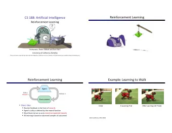
Reinforcement Learning: idea Agent State: s Actions: a Reward: r Environment Basic idea: – Receive feedback in the form of rewards – Agent’s return in long run is defined by the reward function – Must (learn to) act so as to maximize expected return – All learning is based on observed samples of outcomes! 8
The Agent-Environment Interface Agent reward action state r t a t s t r t+ 1 Environment s t+ 1 Agent: Interacts with environment at time t 0 , 1 , 2 , K s S Observes state at step t : t a A(s ) Produces action at step t : t t r R Gets resulting reward: t 1 And resulting next state: s t 1 r t + 1 s t +1 r t +2 s t +2 r t +3 . . . . . . s t +3 s t a a a a t t +1 t +2 t +3 9
Degree of Abstraction Time steps: need not be fixed intervals of real time. Actions: – low level (e.g., voltages to motors) – high level (e.g., accept a job offer) – “mental” (e.g., shift in focus of attention), etc. States: – low‐level “sensations” – abstract, symbolic, based on memory, ... – subjective (e.g., the state of being “surprised” or “lost”). Reward computation: in the agent’s environment (because the agent cannot change it arbitrarily) The environment is not necessarily unknown to the agent, only incompletely controllable. 10
RL as MDP The best studied case is when RL can be formulated as a (finite) Markov Decision Process (MDP), i.e. we assume: A (finite) set of states s S A set of actions (per state) A A model T(s,a,s’) A reward function R(s,a,s’) Markov assumption Still looking for a policy (s) New twist: we don’t know T or R ! – I.e. we don’t know which states are good or what the actions do – Must actually try actions and states out to learn 11
An Example: Recycling robot At each step, robot has to decide whether it should – (1) actively search for a can, – (2) wait for someone to bring it a can, or – (3) go to home base and recharge. Searching is better but runs down the battery; if it runs out of power while searching, it has to be rescued (which is bad). Actions are chosen based on current energy level (states): high, low. Reward = number of cans collected 12
Recycling Robot MDP S high , low search R expected no. of cans while searching A ( high ) search , wait wait R expected no. of cans while waiting A ( low ) search , wait , recharge search wait R R 1, R wait 1— β , —3 β , R search search wait recharge 1, 0 low high wait search 1, R wait search α , R α , R search 1— 13
MDPs and RL Known MDP: offline Solution, no learning Goal Technique Compute V π Policy evaluation Compute V*, * Value / policy iteration Unknown MDP: Model‐Based Unknown MDP: Model‐Free Goal Technique Goal Technique Compute V*, * VI/PI Compute V π Direct evaluation on approximated TD‐learning MDP Compute Q*, * Q‐learning 14
Model-Based Learning Model‐Based Idea: – Learn an approximate model based on experiences – Solve for values, as if the learned model were correct Step 1: Learn empirical MDP model – Count outcomes s’ for each s, a – Normalize to give an estimate of – Discover each when we experience (s, a, s’) Step 2: Solve the learned MDP – For example, use value iteration, as before: 15
Model-Free Learning Model‐Free idea: – Directly learn (approximate) state values, based on experiences Methods (a.o.): I. Direct evaluation Passive: use fixed policy II. Temporal difference learning III. Q‐learning Active: ‘off‐policy’ Remember: this is NOT offline planning! You actually take actions in the world. 16
I: Direct Evaluation Goal: Compute V(s) under given Idea: Average ‘reward to go’ of visits First act according to for several episodes/epochs 1. 2. Afterwards, for every state s and every time t that s is visited: determine the rewards r t … r ⊤ subsequently received in epoch 3. Sample for s at time t = sum of discounted future rewards 𝑡𝑏𝑛𝑞𝑚𝑓 � 𝑆 � 𝑡 � 𝑠 � � 𝛿𝑆 ��� 𝑡′ �𝑆 ⊤ 𝑡 � 𝑠 ⊤ ) given experience tuples <s, (s), r t , s’> 4. Average samples over all visits of s Note: this is the simplest Monte Carlo method 17
Example: Direct Evaluation Observed Episodes Input: Output (Training) Values Policy Episode 1 Episode 2 ‐10 B, east, ‐1, C B, east, ‐1, C A A C, east, ‐1, D C, east, ‐1, D D, exit, +10, D, exit, +10, +8 +4 +10 B C D B C D Episode 3 Episode 4 ‐2 E E E, north, ‐1, C E, north, ‐1, C States C, east, ‐1, D C, east, ‐1, A D, exit, +10, A, exit, ‐10, Assume: = 1 18
Example: Direct Evaluation Observed Episodes Sample computations (Training) A: sample t4‐3 = ‐10 B: sample t1‐1 = ‐1 ‐ 1+ 2 10 = 8 Episode 1 Episode 2 sample t2‐1 = ‐1 ‐ 1+ 2 10 = 8 t1‐1 B, east, ‐1, C B, east, ‐1, C t2‐1 C: sample t1‐2 = ‐1 + 10 = 9 t1‐2 C, east, ‐1, D C, east, ‐1, D t2‐2 sample t2‐2 = ‐1 + 10 = 9 D, exit, +10, D, exit, +10, t1‐3 t2‐3 sample t3‐2 = ‐1 + 10 = 9 sample t4‐2 = ‐1 ‐ 10 = ‐11 Episode 3 Episode 4 D: sample t1‐3 = 10 sample t2‐3 = 10 t4‐1 E, north, ‐1, C E, north, ‐1, C t3‐1 sample t3‐3 = 10 t4‐2 C, east, ‐1, D C, east, ‐1, A t3‐2 E: sample t3‐1 = ‐1 ‐ 1+ 2 10 = 8 D, exit, +10, A, exit, ‐10, t4‐3 t3‐3 sample t4‐1 = ‐1 ‐ 1 ‐ 2 10 = ‐12 Assume: = 1 19
Properties of Direct Evaluation Output Benefits: Values – easy to understand ‐10 – doesn’t require any knowledge of T, R A – eventually computes the correct average values, using just sample transitions +4 +10 +8 B C D Drawbacks: ‐2 – wastes information about state connections E – each state must be learned separately takes a long time to learn If B and E both go to C under this policy, how can their values be different? 20
Recommend
More recommend
Explore More Topics
Stay informed with curated content and fresh updates.
