Approximate Posterior Inference for Differential Equation Models - PowerPoint PPT Presentation

Approximate Posterior Inference for Differential Equation Models Jaeyong Lee Department of Statistics Seoul National University June 24, 2014 jointly with Sarat C. Dass, Universiti Teknologi PETRONAS Kyungjae Lee, Seoul National University and Jonghun Park, Seoul National University.

Outline Introduction of Differential Equation Model First Proposal of Posterior Computation : Laplace + Euler + Grid Sampling Second Proposal of Posterior Computation : Griddy Gibbs Sampling + Euler

Outline Introduction of Differential Equation Model First Proposal of Posterior Computation : Laplace + Euler + Grid Sampling Second Proposal of Posterior Computation : Griddy Gibbs Sampling + Euler

Differential Equations and Statistics Differential equations are widely used. It has many examples. The statistical community has been relatively silent on this area of research.

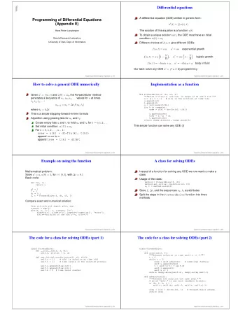
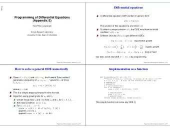
Ordinary Differential Equation Model (Observation Equation) y ( t ) = x ( t ) + ϵ ( t ) , ϵ ( t ) ∼ N ( 0 , σ 2 I p ) , t ∈ [ T 0 , T 1 ] , where ▶ y ( t ) is the p -dimensional vector of observation at time t and ▶ x is the mean function and ϵ ( t ) is the error at time t . ▶ Actual data are observed at discrete times t 1 < t 2 < . . . < t n ∈ [ T 0 , T 1 ] . (Ordinary Differential Equation (ODE)) ˙ x ( t ) = f ( x , u , t : θ ) , t ∈ [ T 0 , T 1 ] , where ▶ f is a smooth p -dimensional function, ▶ u is the input function and ▶ θ is the q -dimensional parameter vector.

SIR Model ˙ x 1 ( t ) = − θ 1 x 1 ( t ) x 2 ( t ) ˙ x 2 ( t ) = θ 1 x 1 ( t ) x 2 ( t ) − θ 2 x 2 ( t ) ˙ x 3 ( t ) = θ 2 x 2 ( t ) x 1 ( t ) : number of the susceptible x 2 ( t ) : number of the infected x 3 ( t ) : number of the recovered : infection rate in ( 0 , 1 ) θ 1 red : x 1 ( t ) , susceptibles : recovery rate rate in ( 0 , 1 ) θ 2 blue : x 2 ( t ) , recovered green : x 3 ( t ) , infected

Lotka-Volterra Equation or Prey-Predator Model ˙ x 1 ( t ) = x 1 ( t )( θ 1 − θ 2 x 2 ( t )) ˙ x 2 ( t ) = − x 2 ( t )( θ 3 − θ 4 x 2 ( t )) x 1 ( t ) : number of the preys x 2 ( t ) : number of the predators : the intrinsic rate of prey population θ 1 increase : the predation rate θ 2 θ 3 : the predator mortality rate θ 4 : the offspring rate of the predator red : x 1 ( t ) , number of preys blue : x 2 ( t ) , number of predators

Computational Methods in Literature-Frequentist Side Nonlinear least squares method with a numerical ODE solver (Bard, 1974). Two step approach (Varah, 1982; Ramsey and Silverman, 2005) Generalized profiling method (Ramsey, Hooker, Campbell and Cao, 2007)

Computational Methods in Literature — Bayesian Side MCMC with numerical solver of ODE (Gelman, Bois and Jiang, 1996; Huang, Liu and Wu, 2006) Collocation Tempering or Smooth functional tempering (Campbell, 2007)

Outline Introduction of Differential Equation Model First Proposal of Posterior Computation : Laplace + Euler + Grid Sampling Second Proposal of Posterior Computation : Griddy Gibbs Sampling + Euler

Differential Equation Model (Observation Model) y i = x ( t i ) + ϵ i , ϵ i ∼ N ( 0 , σ 2 I p ) , i = 1 , 2 , . . . , n , where t 1 < t 2 < . . . < t n . (Differential Equation) x ( t ) = f ( x ( t ) , t | θ ) , θ ∈ Θ ⊂ R q . ˙

Prior Unknowns in the model : θ , σ 2 , x 1 τ 2 = 1 /σ 2 ∼ Gamma ( a , b ) , a , b > 0 . x 1 | τ 2 ∼ N ( µ x 1 , c τ − 2 I p ) , c > 0 . θ ∼ π ( θ ) .

Posterior π ( θ, τ 2 , x 1 | y n ) p ( y n | θ, τ 2 , x 1 ) π ( x 1 | τ 2 ) π ( τ 2 ) π ( θ ) ∝ n | τ − 2 2 π I p | − 1 / 2 e − τ 2 2 || y i − x i ( θ, x 1 ) || 2 � = i = 1 2 c || x 1 − µ x 1 || 2 × b a Γ( a )( τ 2 ) a − 1 e − b τ 2 × π ( θ ) ×| 2 π c τ − 2 I p | − 1 / 2 e − τ 2 2 ( n + 1 ) p + a − 1 e − τ 2 c || x 1 − µ x 1 || 2 + 2 b ) × π ( θ ) , 1 2 ( ng n ( x 1 ,θ )+ 1 ( τ 2 ) ∝ where y n = ( y 1 , y 2 , . . . , y n ) i = 1 || y i − x i ( θ, x 1 ) || 2 and � n g n ( x 1 ) = g n ( x 1 , θ ) = 1 n || x || denotes the Euclidean norm of the vector x .

First Proposal : Laplace approximation and grid sampling Unknowns in the model : θ , σ 2 , x 1 Marginalization Step : Laplace approximation and Euler method to eliminate x 1 from the posterior Sampling θ and σ 2 ▶ Sampling θ : grid sampling ▶ Sampling τ 2 = 1 /σ 2 : sampling from gamma distribution

Marginalization of x 1 Using Tierney and Kadane (1986), � L ( θ, τ 2 ) π ( x 1 | τ 2 ) L ( θ, τ 2 , x 1 ) dx 1 = x 1 ) + 2 ( τ 2 ) np / 2 e − τ 2 2 u ( θ ) det ( n ¨ c I p ) − 1 / 2 ( 1 + O ( n − 3 / 2 )) , g n (ˆ ∝ where ∂ 2 g n ( x 1 ) ¨ = g n ( x 1 , θ ) ∂ x 2 1 ng n ( x 1 , θ ) + 1 c ∥ x 1 − µ x 1 ∥ 2 � � ˆ ˆ x 1 = x 1 ( θ ) = argmin x 1 x 1 ) + 1 x 1 − µ x 1 || 2 . ng n (ˆ c || ˆ u ( θ ) =

x 1 ) + 2 π ( θ, τ 2 | y n ) ∝ π ( θ ) × det ( n ¨ c I p ) − 1 / 2 g n (ˆ np 2 + a − 1 e − τ 2 ( 1 × ( τ 2 ) 2 u ( θ )+ b ) .

π ( τ 2 | θ, y n ) τ 2 | θ, y n ∼ Gamma ( a ∗ , b ∗ ) , where np a ∗ = 2 + a 1 b ∗ = 2 u ( θ ) + b .

π ( θ | y n ) � π ( θ, τ 2 | y n ) d τ 2 π ( θ | y n ) = π ( θ ) ∝ c I p ) 1 / 2 . np ( 1 2 + a det ( n ¨ x 1 ) + 2 g n (ˆ 2 u ( θ ) + b ) Sampling θ is done by grid sampling.

Second Proposal : griddy Gibbs sampling Unknowns in the model : θ , σ 2 , x 1 Sampling x 1 and θ : griddy Gibbs Sampling τ 2 = 1 /σ 2 : sampling from gamma distribution

Newton’s Law of Cooling (Differential Equation) ˙ x ( t ) = θ 1 [ x ( t ) − θ 2 ] , t ≥ 0 , where ▶ x ( t ) is the temperature of an object in Celcius; ▶ θ 2 is the temperature of the environment; and ▶ θ 1 is the proportionality constant. The analytic form of the solution is known : x ( t ) = θ 2 − ( θ 2 − x 1 ) e θ 1 t , t ≥ t 1 > = 0 .

Quality of Laplace Approximation Figure : The true posterior density and approximate posterior density with Laplace approximation when sample size n = 20.

Step Size of Euler Method

FitzHugh-Nagumo Model FitzHugh-Nagumo Model is a differential equation for spike potential of giant axon of squid neurons. (Differential Equation) θ 3 [ x 1 ( t ) − 1 3 x 3 ˙ x 1 ( t ) = 1 ( t ) + x 2 ( t )] − 1 ˙ x 2 ( t ) = [ x 1 ( t ) − θ 1 + θ 2 x 2 ( t )] , θ 3 where ▶ x 1 ( t ) (voltage) is the voltage across an membrane at time t , ▶ x 2 ( t ) (recovery) is the outward currents. ▶ To get meaningful behavior, 1 − 2 3 θ 2 < θ 1 < 1 , 0 < θ 2 < 1 and θ 2 < θ 2 3 should be satisfied.

Step sizes of Euler Method and Approximate Posteriors

Convergence of Approximate Posterior In actual computation, to improve accuracy of the Euler method, we divide [ t i − 1 , t i ] into m intervals. Under certain conditions, for all θ and σ 2 , m →∞ π m ( θ, τ 2 | y n ) = π 0 ( θ, τ 2 | y n )( 1 + O ( n − 3 / 2 )) . lim

Outline Introduction of Differential Equation Model First Proposal of Posterior Computation : Laplace + Euler + Grid Sampling Second Proposal of Posterior Computation : Griddy Gibbs Sampling + Euler

Griddy Gibbs Sampling The posterior of θ and x 1 , π ( θ, x 1 | y ) , is approximated by discrete distribution whose probabilities are proportional to π ( θ, x 1 | y ) . When the dimension of θ and x 1 is not small, we apply griddy Gibbs sampling or Gibbs sampling to the discrete approximation of the posterior. When some of the parameters of the posterior are highly correlated, we use blocked Gibbs.

Calcium oscillation model x 1 ( t ) = θ 1 + θ 2 x 1 ( t ) − θ 5 x 1 ( t ) x 2 ( t ) ˙ x 1 ( t ) + θ 6 − θ 7 x 1 ( t ) x 3 ( t ) x 1 ( t ) + θ 8 θ 9 x 2 ( t ) ˙ x 2 ( t ) = θ 3 x 1 ( t ) − x 2 ( t ) + θ 10 θ 11 x 3 ( t ) x 3 ( t ) = θ 4 x 1 ( t ) − ˙ x 3 ( t ) + θ 12 x 1 : the concentration of active subunit of the G-protein x 2 : the concentration of activated form of PLC x 3 : the concentration of cytosolic Calcium

Estimation and prediction

Thank You!