ANT-INSPIRED DENSITY ESTIMATION VIA RANDOM WALKS Nancy Lynch, - PowerPoint PPT Presentation
ANT-INSPIRED DENSITY ESTIMATION VIA RANDOM WALKS Nancy Lynch, Cameron Musco, Hsin-Hao Su BDA 2016 July, 2016 Chicago, Illinois 1. Introduction Ants appear to use estimates of colony density (number of ants per unit area), in solving
ANT-INSPIRED DENSITY ESTIMATION VIA RANDOM WALKS Nancy Lynch, Cameron Musco, Hsin-Hao Su BDA 2016 July, 2016 Chicago, Illinois
1. Introduction • Ants appear to use estimates of colony density (number of ants per unit area), in solving typical ant colony problems: • Searching for a new nest: Ants decide to accept a nest when they detect that the ant density in the nest has become sufficiently high [Pratt 05]. • Engaging or retreating: Ants may decide to engage or retreat based on relative density of their own vs. an enemy colony [Adams 90] . • Task allocation: Ants may choose tasks based on densities of ants already allocated to various tasks [Gordon 99], [Schafer, Holmes, Gordon 06]. • Estimate density based on encounter rates [Gordon, Paul, Thorpe 93], [Pratt 05]. • Q: How might this work, and how accurate are the estimates?
Density estimation in distributed systems • Similarly, agents in distributed systems could use density estimates in solving distributed computing problems: • Robot swarms: • Robots can determine the frequency of certain properties within the swarm, such as detecting an environment event. • Robots can allocate themselves to tasks, or distribute themselves evenly around an area. • Social networks: • One could estimate the size of a network by launching agents and observe how frequently they encounter others [Katzir, Liberty, Somekh 11]. • Estimating density is equivalent to: • Estimating the number of agents, if the area is known, or • Estimating the area, if the number of agents is known.
How we got interested: • Distributed House-Hunting in Ant Colonies [Ghaffari, Lynch, Musco, Radeva PODC 15]. • Algorithm: Ants evaluate nest desirability by determining numbers of ants in the nests and how the numbers change over time. • 𝑃(log 𝑜) time until termination. • Approximately matching lower bound, Ω(log 𝑜). • This assumes that an ant can determine the number of ants in a nest precisely. • Typical sort of assumption for distributed algorithms. • Not realistic for ants: they cannot count precisely, they move,… • Makes the algorithm too fragile, for a biological algorithm. • Led us to study approximate counting, which could be implemented by estimating density.
Our latest algorithm • Ant-Inspired Density Estimation via Random Walks [Lynch, Musco, Su PODC 16, arXiv] • Uses encounter rates, as suggested by [Gordon, Paul, Thorpe 93], [Pratt 05]. • Specifically: • Ants wander in a 2-D plane, using independent random walks. • Each ant determines its number of encounters per unit time. • Uses that as a density estimate (number of ants per unit area). • Notes: • This assumes that an ant can count its number of encounters, although ants cannot count precisely. • Actually, the algorithm is not so fragile---approximate counting should be good enough. • But for now, just pretend an ant can count its encounters precisely.
Our algorithm • Geometry is important for our results. • 2-dimensional plane. • Discretize space: Describe the plane as a grid, with ants on the nodes. • Then fold the grid into a torus:
Our algorithm • Discretize time: Synchronous rounds. • Algorithm: • In each round, each ant takes a step in a random direction, sees how many ants it encounters at the new position, and adds this number to a running 𝑑𝑝𝑣𝑜𝑢. • After 𝑢 rounds, it outputs the value of the ratio /0123 . 3 2 • Claim: This is a good estimate for the ant density 𝑒 = 6786 . • Q: How good? • A: With “high probability”, the estimate is correct to within a small inaccuracy 𝜗, provided that the number 𝑢 of rounds is at least a certain constant times ; ( ; <= > times log <= ) .
� � 2. Model and Problem • Torus grid, 𝐵 locations, 𝐵 by 𝐵 . • Ants start at (uniformly, independently chosen) random locations. • Then they work in synchronous rounds. • At every round, each ant can choose (deterministically or probabilistically) to move one step in any direction, or to not move. • In every round, each ant can detect how many other ants have reached the same grid location in the same round. • It can also remember these numbers, e.g., by accumulating them in a single internal 𝑑𝑝𝑣𝑜𝑢 variable.
The Density Estimation problem • Each ant should continually output its latest estimate of the density 𝑒 = 𝑜/𝐵 , where 𝑜 is the total number of ants and 𝐵 is the total number of grid points in the torus. • Ants are not assumed to know 𝑜 or 𝐵 , and don’t need to determine these---just the ratio. • But if they happen to know 𝑜 or 𝐵 , the density estimate yields an estimate of the other.
3. The Algorithm • Simplest possible! • Ants are initially randomly placed at grid locations. • Algorithm for ant 𝑏 C : • Local variables: • 𝑑𝑝𝑣𝑜𝑢 , initially 0 • 𝑢𝑗𝑛𝑓, initially 0 • At every round: • Set 𝑢𝑗𝑛𝑓 ∶= 𝑢𝑗𝑛𝑓 + 1. • Move in any of the four directions, each with probability ¼. • See how many other ants have reached the same grid location in the same round. • Add that number to 𝑑𝑝𝑣𝑜𝑢 . M0123 • Output estimate 𝑓𝑡𝑢 = 3CN8 .
The Algorithm • Algorithm for ant 𝑏 C : • At every round: • Set 𝑢𝑗𝑛𝑓 ∶= 𝑢𝑗𝑛𝑓 + 1. • Move in any of the four directions, each with probability ¼. • See how many other ants have reached the same grid location in the same round. • Add that number to 𝑑𝑝𝑣𝑜𝑢 . M0123 • Output estimate 𝑓𝑡𝑢 = 3CN8 . M0123 • Q: Why is 3CN8 a plausible estimate for density 𝑒 = 𝑜/𝐵 ? • 𝑒 = 𝑜/𝐵 is the expected number of ants at any particular location at any particular time. M0123 3CN8 is the average number any particular ant sees at any time. • • Those are the same.
4. The Analysis • How does this behave? • Theorem 1: The expected value of any ant’s estimate is equal to the actual ant density 𝑒 = 𝑜/𝐵 . • As we just argued. • But we also want a high-probability result: With “high probability”, the estimate is correct to within 𝜗, provided that the number 𝑢 of rounds is “sufficiently large”. • Having the right expectation doesn’t automatically imply high probability that our estimate is close to the expectation.
Analysis • High-probability result: With “high probability”, the estimate is correct to within 𝜗, provided that the number 𝑢 of rounds is “sufficiently large”. • In completely-connected graphs, a high- probability result follows easily: • Any ant is equally likely to go anywhere at each round. • Occurrences of encounters are essentially independent at each round. • Standard probability results (Chernoff bounds) yield a good high-probability result: • Theorem 2 (for complete graphs): With “high probability”, the estimate is correct to within 𝜗, provided that the number 𝑢 of ; <= > . rounds is at least a certain constant times
Analysis • We say that the complete graph has fast mixing time, meaning there is little correlation between successive locations for an ant. • On the other hand, the torus grid graph has slow mixing time--- strong correlation between successive locations for an ant. • Thus, when ant 𝑏 C encounters ant 𝑏 O in some round, it is likely to encounter it again in the following rounds. • High variance in time between successive encounters. • Still, we obtain: • Theorem 3 (for torus grid graphs): With “high probability”, the estimate is correct to within 𝜗, provided that the number 𝑢 of ; ; <= > times log ( <= ) . rounds is at least a certain constant times
Analysis • Theorem 3 (for torus grid graphs): With “high probability”, the estimate is correct to within 𝜗, provided that the number 𝑢 of rounds is at least a ; ; <= > times log ( <= ) . constant times • Proof: • Calculations, based on bounding the moments of the distribution of numbers of encounters. • See [Lynch, Musco, Su, PODC 16, arXiv] for details. • Key Lemma 4 (Re-collision bound): If 𝑏 C and 𝑏 O collide in round 𝑠, then the probability that they collide again in round 𝑠 + 𝑛 is ; ; (approximately) Θ NR; + 𝑃 S .
5. Discussion • We have shown that a very simple random exploration algorithm for the 2-dimensional plane gives accurate estimates of colony density, even though collisions at successive rounds are not independent. • May be useful for understanding insect behavior: • Searching for a new nest • Engaging or retreating • Allocating ants to tasks • And for distributed computing: • Robot swarms • Estimating the size of a large social network • See [Lynch, Musco, Su 16] for some examples.
� Results: Other graph classes graphs • Density estimation for other classes of graphs: • Rings • Higher-dimensional tori • Regular expanders • Hypercubes • The key in each case is a re-collision bound, e.g., for a ring: • Key Lemma (Re-collision bound): If 𝑏 C and 𝑏 O collide in round 𝑠, then the probability that they collide again in round 𝑠 + 𝑛 is ; ; (approximately) Θ R; + 𝑃 S . N • We use a general result that converts re-collision bounds to bounds for density estimation.
Recommend
More recommend
Explore More Topics
Stay informed with curated content and fresh updates.
