Announcements Wednesday, August 29 WeBWorK 2.1 due today at - PowerPoint PPT Presentation
Announcements Wednesday, August 29 WeBWorK 2.1 due today at 11:59pm. The first quiz is on Friday, during recitation. It covers through section 2.1 . Quizzes mostly test your understanding of the homework. Quizzes last 10 minutes.
Announcements Wednesday, August 29 ◮ WeBWorK 2.1 due today at 11:59pm. ◮ The first quiz is on Friday, during recitation. It covers through section 2.1 . ◮ Quizzes mostly test your understanding of the homework. ◮ Quizzes last 10 minutes. Books, calculators, etc. are not allowed. ◮ There will generally be a quiz every Friday when there’s no midterm. ◮ Check the schedule if you want to know what will be covered. ◮ My office is Skiles 244 and Rabinoffice hours are: Mondays, 12–1pm; Wednesdays, 1–3pm. ◮ Your TAs have office hours too. You can go to any of them. Details on the website. ◮ Many other resources are also contained in the “Help” tab of the master website. This includes Math Lab (not to be confused with MyMathLab), a free one-on-many tutoring service, open for many hours most days, provided by the School of Math.
(Reduced) Row Echelon Form Review from last time A matrix is in row echelon form if 1. All zero rows are at the bottom. 2. Each leading nonzero entry of a row is to the right of the leading entry of the row above. 3. Below a leading entry of a row, all entries are zero . A matrix is in reduced row echelon form if it is in row echelon form, and in addition, 4. The pivot in each nonzero row is equal to 1. 5. Each pivot is the only nonzero entry in its column. Row echelon form: Reduced row echelon form: 1 0 0 ⋆ ⋆ ⋆ ⋆ ⋆ ⋆ ⋆ 0 0 1 0 ⋆ ⋆ ⋆ ⋆ ⋆ ⋆ 0 0 0 0 0 0 1 ⋆ ⋆ ⋆ 0 0 0 0 0 0 0 0 0 0 ⋆ = pivots
Row Reduction: Theorem Theorem Every matrix is row equivalent to one and only one matrix in reduced row echelon form. We’ll give an algorithm, called row reduction or Gaussian elimination , which demonstrates that every matrix is row equivalent to at least one matrix in reduced row echelon form. Note: Like echelon forms, the row reduction algorithm does not care if a column is augmented: ignore the vertical line when row reducing. The uniqueness statement is interesting—it means that, nomatter how you row reduce, you always get the same matrix in reduced row echelon form. (Assuming you only do the three legal row operations.) (And you don’t make any arithmetic errors.) Maybe you can figure out why it’s true!
Row Reduction Algorithm Step 1a Swap the 1st row with a lower one so a leftmost nonzero entry is in 1st row (if necessary). Step 1b Scale 1st row so that its leading entry is equal to 1. Step 1c Use row replacement so all entries below this 1 are 0. Step 2a Swap the 2nd row with a lower one so that the leftmost nonzero entry is in 2nd row. Step 2b Scale 2nd row so that its leading entry is equal to 1. Step 2c Use row replacement so all entries below this 1 are 0. Step 3a Swap the 3rd row with a lower one so that the leftmost nonzero entry is in 3rd row. etc. Last Step Use row replacement to clear all entries above the pivots, starting with the last pivot (to make life easier). Example 0 − 7 − 4 2 2 4 6 12 3 1 − 1 − 2 [animated]
Row Reduction Example 0 − 7 − 4 2 2 4 6 12 3 1 − 1 − 2
Row Reduction Example, continued 1 2 3 6 0 − 5 − 10 − 20 0 − 7 − 4 2 Note: Step 2 never messes up the first (nonzero) column of the matrix, because it looks like this: 1 ⋆ ⋆ ⋆ 0 “Active” row ⋆ ⋆ ⋆ 0 ⋆ ⋆ ⋆
Row Reduction Example, continued 1 2 3 6 0 1 2 4 0 0 10 30
Row Reduction Example, continued Success! The reduced row echelon form is 1 0 0 1 x = 1 0 1 0 − 2 = y = − 2 ⇒ 0 0 1 3 z = 3
Recap Clear down Get a 1 here Get a 1 here Clear down 1 1 1 ⋆ ⋆ ⋆ ⋆ ⋆ ⋆ ⋆ ⋆ ⋆ ⋆ ⋆ ⋆ ⋆ 0 0 1 ⋆ ⋆ ⋆ ⋆ ⋆ ⋆ ⋆ ⋆ ⋆ ⋆ ⋆ ⋆ ⋆ 0 0 ⋆ ⋆ ⋆ ⋆ ⋆ ⋆ ⋆ ⋆ ⋆ ⋆ ⋆ ⋆ ⋆ ⋆ 0 0 ⋆ ⋆ ⋆ ⋆ ⋆ ⋆ ⋆ ⋆ ⋆ ⋆ ⋆ ⋆ ⋆ ⋆ (maybe these are already zero) Get a 1 here Clear down Matrix is in REF 1 1 1 1 ⋆ ⋆ ⋆ ⋆ ⋆ ⋆ ⋆ ⋆ ⋆ ⋆ ⋆ ⋆ 0 1 0 1 0 1 0 1 ⋆ ⋆ ⋆ ⋆ ⋆ ⋆ ⋆ ⋆ 0 0 0 0 0 0 0 0 0 1 0 0 0 1 ⋆ ⋆ 0 0 0 0 0 0 0 0 0 0 0 0 0 ⋆ ⋆ ⋆ Clear up Clear up Matrix is in RREF 1 1 0 1 0 0 ⋆ ⋆ ⋆ ⋆ ⋆ ⋆ 0 1 0 1 0 0 1 0 Profit? ⋆ ⋆ ⋆ ⋆ 0 0 0 1 0 0 0 1 0 0 0 1 0 0 0 0 0 0 0 0 0 0 0 0
Row Reduction Another example The linear system 2 x + 10 y = − 1 gives rise to the matrix 3 x + 15 y = 2 Let’s row reduce it: [interactive row reducer] � 2 � 10 − 1 3 15 2 The row reduced matrix � 1 � 5 0 corresponds to the x + 5 y = 0 0 0 1 inconsistent system 0 = 1.
Inconsistent Matrices Question What does an augmented matrix in reduced row echelon form look like, if its system of linear equations is inconsistent? An augmented matrix corresponds to an inconsistent system of equations if and only if the last (i.e., the augmented) column is a pivot column.
Section 2.3 Parametric Form
Another Example The linear system � 2 � 2 x + y + 12 z = 1 1 12 1 gives rise to the matrix . x + 2 y + 9 z = − 1 1 2 9 − 1 Let’s row reduce it: [interactive row reducer] � 2 � 1 12 1 1 2 9 − 1 The row reduced matrix � 1 � x + 5 z = � 1 0 5 1 corresponds to the 0 1 2 − 1 linear system y + 2 z = − 1
Another Example Continued The system x + 5 z = 1 y + 2 z = − 1 comes from a matrix in reduced row echelon form. Are we done? Is the system solved? Yes! Rewrite: x = 1 − 5 z y = − 1 − 2 z For any value of z , there is exactly one value of x and y that makes the equations true. But z can be anything we want ! So we have found the solution set: it is all values x , y , z where x = 1 − 5 z y = − 1 − 2 z for z any real number. ( z = z ) This is called the parametric form for the solution. [interactive picture]
Free Variables Definition Consider a consistent linear system of equations in the variables x 1 , . . . , x n . Let A be a row echelon form of the matrix for this system. We say that x i is a free variable if its corresponding column in A is not a pivot column. Important 1. You can choose any value for the free variables in a (consistent) linear system. 2. Free variables come from columns without pivots in a matrix in row echelon form. In the previous example, z was free because the reduced row echelon form matrix was � 1 � 0 5 4 . 0 1 2 − 1 In this matrix: � 1 � 0 ⋆ ⋆ ⋆ 0 0 1 ⋆ ⋆ the free variables are x 2 and x 4 . (What about the last column?)
One More Example The reduced row echelon form of the matrix for a linear system in x 1 , x 2 , x 3 , x 4 is � 1 � 0 0 3 2 0 0 1 4 − 1 The free variables are x 2 and x 4 : they are the ones whose columns are not pivot columns. This translates into the system of equations � x 1 + 3 x 4 = 2 x 1 = 2 − 3 x 4 = ⇒ x 3 + 4 x 4 = − 1 x 3 = − 1 − 4 x 4 . What happened to x 2 ? What is it allowed to be? Anything! The general solution is for any values of x 2 and x 4 . The boxed equation is called the parametric form of the general solution to the system of equations. It is obtained by moving all free variables to the right-hand side of the =.
Yet Another Example The linear system x + y + z = 1 has matrix form This is in reduced row echelon form. The free variables are y and z . The parametric form of the general solution is Rearranging: ( x , y , z ) = (1 − y − z , y , z ) , where y and z are arbitrary real numbers. This was an example in the second lecture! [interactive]
Poll
Trichotomy There are three possibilities for the reduced row echelon form of the augmented matrix of a linear system. 1. The last column is a pivot column. In this case, the system is inconsistent . There are zero solutions, i.e. the solution set is empty . Picture: 1 0 0 0 1 0 0 0 1 2. Every column except the last column is a pivot column. In this case, the system has a unique solution . Picture: 1 0 0 ⋆ 0 1 0 ⋆ 0 0 1 ⋆ 3. The last column is not a pivot column, and some other column isn’t either. In this case, the system has infinitely many solutions, corresponding to the infinitely many possible values of the free variable(s). Picture: � 1 � 0 ⋆ ⋆ ⋆ 0 0 1 ⋆ ⋆
Recommend
More recommend
Explore More Topics
Stay informed with curated content and fresh updates.

